2 Introduction

Tide gauge data is crucial for storm surge modeling. The validation of hydrodynamic models relies in part on the comparison of model results to observed tidal water levels. Model parameters can be calibrated to reproduce tidal flow more accurately. The region surrounding the Ganges-Brahmaputra-Meghna (GBM) Delta is particularly vulnerable to storm surge events (Dube et al., 1997). The context of storm surge threats makes tidal analysis especially relevant for the region.

Tazkia et al. (2017) use a barotropic numerical model to mimic the effect of meteorologically induced seasonal sea level variations onto tidal amplitudes. They use sea level data measured by tide gauges to validate their model, performing classical harmonic analysis on sliding windows of 2 months length to obtain a temporally varying amplitude of the semidiurnal lunar constituent M2.

Before that, Müller et al. (2014) studied the seasonal cycle of M2 produced by a global numerical ocean model using two different methods. In the first method, harmonic analysis is applied to sliding windows of 32 days of water level records. The second method builds on the concepts of classical harmonic analysis and interprets the seasonal modulation of M2 as induced by a fictitious celestial body (or satellite). This has the conceptual advantage that M2 can be expressed by true harmonic constants, which are by definition independent of time, but requires the introduction of additional constituents to express the temporal modulation. The practice of defining a "meteorological constituent" which modulates M2 at an annual frequency, goes back at least to Corkan (1934) (see Müller et al., 2014, for reference).

We summarized the method of Corkan (1934) and Müller et al. (2014) in more detail in a previous post. In that post, we described the results of harmonic analysis of 6 tide gauges in the north-eastern Bay of Bengal, using water level time series of 366 days length. The preprocessed hourly and daily water level data was retrieved from the Joint Archive for Sea Level (JASL, see Caldwell et al. 2015), maintained by the University of Hawaii Sea Level Center (UHSLC) . We showed figures of

amplitudes of harmonic constituents
seasonal variation of sea level and predictions by the solar annual constituent

All previous figures can be accessed from this list in our previous post.

In the present blog post, we measure the seasonal variation of M2 amplitude with the two methods used by Müller et al. (2014).

3 Methods

3.1 Observations and data

A map of the 6 tide gauge stations is shown in the companion blog post. UHSLC maintains an archive of research-quality water level data with hourly and daily resolution, containing (among many others) the following stations shown on the map:

Table 1: Table 1: List of UHSLC tide gauge stations with time series data
UHSLC station ID	UHSLC station name	Country
124	Chittagong	Bangladesh
134	Hiron Point	Bangladesh
136	Cox's Bazaar	Bangladesh
138	Charchanga	Bangladesh
139	Khepupara	Bangladesh
907	Akyab (Sittwe)	Myanmar

Note that we do not use any data from stations Khal #10 and Teknaf. The tide gauge data is preprocessed by UHSLC (Caldwell et al., 2015) and/or possibly other third parties (see acknowledgements6 ). IOC (1992) describe the standardized data processing and quality assurance methodology followed to produce the Research Quality dataset archived by the NOAA National Centers for Environmental Information as the Joint Archive for Sea Level (JASL, see Caldwell et al. 2015). The quality assessment policy (FTP link) states that assessment is mostly based on residuals (observed data minus predicted tides) of hourly data. IOC (1992) state that the hourly data is computed from the high-frequency data delivered by the instrument via a three-point Hanning filter. IOC (1992) further state that the filter was chosen to minimize aliasing from subsampling and to minimize the attenuation of the tides. The archive also contains daily time series. Caldwell (2015) describes the two-step tidal filtering procedure for computation of the daily values. In a first step, dominant diurnal and semi-diurnal tidal components are removed from the quality controlled hourly values. Secondly, a 119-point convolution filter is applied to remove the remaining high frequency energy and to prevent aliasing.

3.2 Methods for assessing M2 amplitude variation

We mostly follow Müller et al. (2014), who use two methods to quantify the seasonal cycle of M2 amplitude. For the first method, the time series are split into monthly segments of 32 days length, on which we perform harmonic analysis to obtain M2. The second method is based on the work of Corkan (1934) and determines the harmonic constants associated with modulating side frequencies of M2. Müller et al. (2014) use tide gauge records of 20 years length, we use records of only 366 days length. Tazkia et al. (2017) study the M2 amplitude variation in the north-eastern Bay of Bengal. They use method 1, but with a sliding window of two months.

We use the term amplitude modulation in this blog post rather loosely, and possibly in a way that is inconsistent with the general literature on signal processing. For a motivation of method 2, let the composite sea level predicted by the tidal constituents M2, \(\alpha_2\) and \(\beta_2\) be defined as

\begin{equation} \zeta_{comp}(t) := \sum_{i=1..3}a_i\cos{\left(2\pi f_i t - \phi_{i}\right)},\label{eq:eq1} \end{equation}

where \(f_i\) is the respective constituent's frequency and the amplitude \(a_i\) and phase \(\phi_i\) are the results of classical tidal harmonic analysis of 366-day intervals as described in the companion blog post. Below we refer to quantities associated with this composite simply as M2+\(\alpha_2\)+\(\beta_2\), and it should be clear from the context whether sea level or amplitude etc. is meant.

The constituents used in Eq. \eqref{eq:eq1} have frequencies

\begin{gather*} f_1 := f_{M2} := 2f_L \\ f_2 := f_{\alpha_2} := 2f_L-f_{SA} \\ f_3 := f_{\beta_2} := 2f_L+f_{SA}, \end{gather*}

where \(f_L\) is the frequency corresponding to the period of a mean lunar day, and \(f_{SA}\) is the frequency of the solar annual constituent. In the discussion section of the companion blog post, we take note of apparently inconsistent definitions of SA in the literature, which in turn seem to give rise to inconsistent definitions of \(\alpha_2\) and \(\beta_2\) on the one hand, and constituents \(MA_2\) and \(Ma_2\) used e.g. by Corkan (1934) on the other hand (see Müller et al., 2014, and references therein), all of which are apparently attributed a similar physical significance at the time scales under consideration.

A classical result for amplitude modulation in signal processing may be obtained from \eqref{eq:eq1} under certain conditions. Sufficient conditions are that (1) all \(\phi_i\) vanish and (2) that \(a_2=a_3\). As shown in Appendix B, Eq. \eqref{eq:eq1} then simplifies to

\begin{gather*} \zeta_{comp}(t) = A(f_{SA},t)\cos{(2\pi f_{M2})}, \end{gather*}

where

\begin{gather*} A(f_{SA},t) = a_{M2} + 2a_{\alpha_2,\beta_2}\cos{\left(2\pi f_{SA}t\right)} \end{gather*}

Note that \(A(f_{SA},t)\) is independent of the carrier frequency \(f_{M2}\). The amplitude of the modulated M2 signal varies with annual frequency \(f_{SA}\). Importantly, the maximum (minimum) amplitude of the composite can simply be obtained by adding (subtracting) twice the modulation amplitude to (from) the carrier amplitude. Initial attempts by the author to reproduce Eq. (22) of Müller et al. (2014), where all phases and amplitudes are generally allowed to differ, were unsuccessful, and we speculate that they may contain an error. To avoid possibly tedious analytical computations, we simply estimate the variations of amplitude of the composite function by numerical methods. We compute the range of the composite in a sliding 14-hour window and divide it by two.

3.3 Harmonic analysis software

We use the SLP64 software package distributed by the University of Hawaii Sea Level Center, which includes the IOS Tidal Package written by Foreman (1977). The IOS Tidal Package in turn is based on the work by Godin (1972) and Godin and Taylor (1973). The related T_Tide MATLAB package of Pawlowicz et al. (2002) is based on the IOS Tidal Package but includes methods to compute confidence intervals and signal-to-noise ratios. Originally, a secondary motivation of this blog post (and the companion blog post) was to collect useful notes on the use of the IOS Tidal Package and T_Tide and conflate them with a practical application to data from the Bay of Bengal. However, the blog post became too long and we moved the software notes into a separate post.

4 Results

4.1 Listing of figures

Seasonal variation of M2 amplitude

Chittagong (Chattogram) 124a
Hiron Point 134a
Cox's Bazaar 136a
Charchanga 138a
Khepupara 139a
Akyab (Sittwe) 907a

M2 amplitude as a function of sea level anomaly

Chittagong (Chattogram) 124a
Hiron Point 134a
Cox's Bazaar 136a
Charchanga 138a
Khepupara 139a
Akyab (Sittwe) 907a

Amplitudes of tidal constituents (Chittagong only):

Chittagong 124a

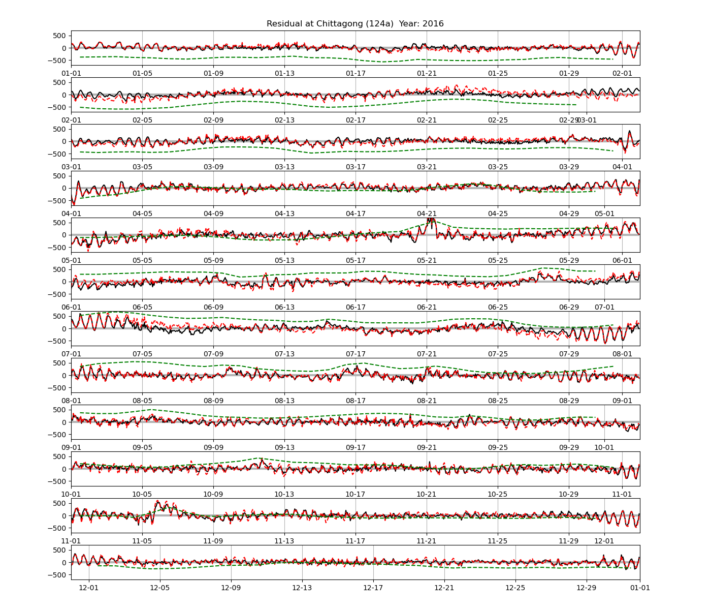
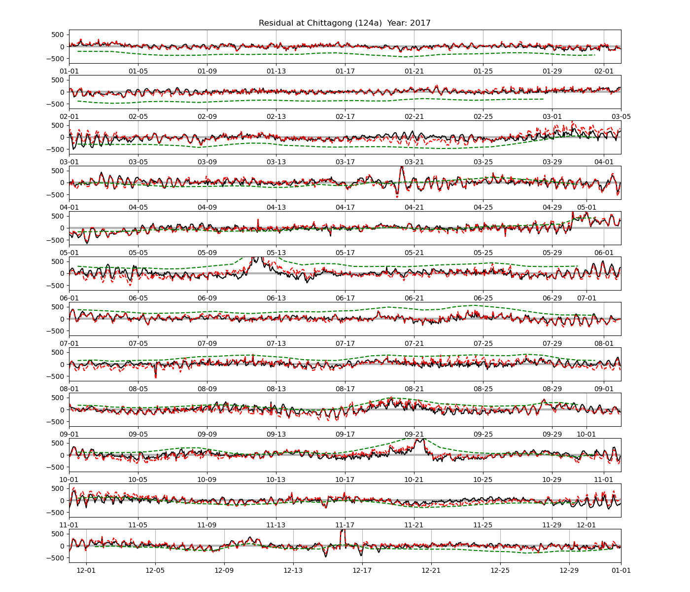
Residuals of harmonic analysis (Chittagong, year 2008 only):

Station name	Station id	Link to plot of residuals
Chittagong	124a	2008 , 2010 , 2012 , 2016 , 2017

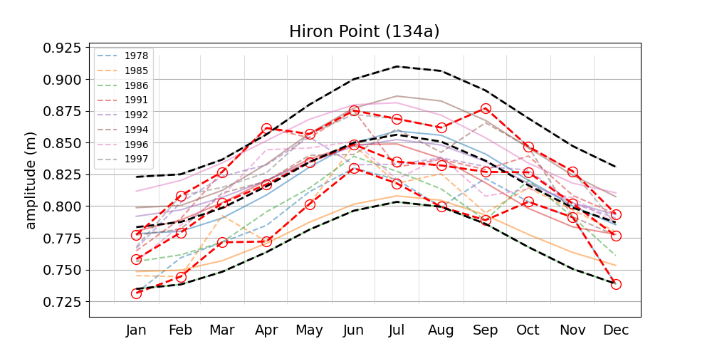
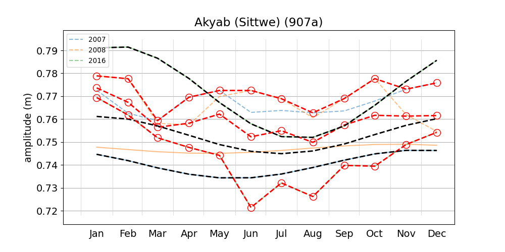
Figure 1 shows a comparison between the two methods for computing M2 amplitude variations. The data shown here is for the Chittagong station (map), and plots for the remaining stations can be accessed from the list. The composite M2+\(\alpha_2\)+\(\beta_2\) amplitude was estimated numerically as half of the tidal range within a 14 hour interval (see section 3 ), and then averaged over the calendar month. The multi-year mean of the two methods differ by less than 10 cm throughout the year and range from about 1.5 m in February to about 1.95 m in August, i.e. roughly 25 percent of the annual mean value. The sum of the multi-year mean amplitude of the tidal constituents \(\alpha_2\) and \(\beta_2\) is about 0.25 m (see the corresponding figure in the companion blog post), and their composite (denoted as \(\alpha_2\)+\(\beta_2\)) has therefore a maximum range of about 0.5 m throughout the year (i.e. at times of positive interference). Figure 5 shows the result for the tide gauge at Hiron Point, which may be compared with Fig. 2 of Tazkia et al. (2017). The maximum difference between the multi-year mean amplitudes computed with the two methods is about 0.025 m throughout the year. The seasonal variation of amplitude is lower than in Chittagong, both in absolute and relative terms, consistent with the result of Tazkia et al. (2017). The multi-year mean composite amplitude ranges from about 0.78 m to 0.86 m, i.e. about 8 cm throughout the year. The sum of adding the multi-year mean amplitude of the tidal constituents \(\alpha_2\) and \(\beta_2\) yields about 8.9 cm (see here), and their composite \(\alpha_2\)+\(\beta_2\) has therefore a maximum range of 17.8 cm. Contrary to Chittagong, the maximum range of \(\alpha_2\)+\(\beta_2\) is not a good estimate for the M2 amplitude range at Hiron Point. To see how this may be related to phase shifts between the \(\alpha_2\)+\(\beta_2\) on the one hand, and M2 on the other hand, compare the corresponding figures in the discussion section of our companion blog post.

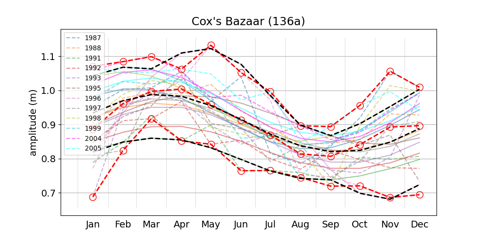
The composite M2+\(\alpha_2\)+\(\beta_2\) amplitude is low in summer and high in winter at 4 out of 6 stations. Cox's Bazaar (Figure 6) and Akyab (Figure 9) are exceptions, with approximately inverse behaviour, i.e high amplitude in summer and low amplitude in winter. Both stations are located on the east coast of the Bay of Bengal (see map), where the continental shelf is steeper than at the other stations.

Note that the metadata sheet of the tide gauge at Cox's Bazaar indicates that the cause of large periodic fluctuations in the residual is unclear, and that they could be due to the timing of the tide gauge.

Amplitude modulation — Figure 1: The **center black** line shows the multi-year mean of the composite M2+\(\alpha_2\)+\(\beta_2\) amplitude (in meters) of sea level predictions for the Chittagong tide gauge. The **upper and lower black** lines show the multi-year maximum and minimum of the composite amplitude. The **center red dashed** line shows the multi-year mean of the M2 amplitude computed from harmonic analysis of a 32 days window starting at the beginning of each calendar month (with the exception of December). For December, the last day of November was prepended to the time series. The **upper and lower red dashed** lines show the multi-year maximum and minimum of the 32-day M2 amplitude. The **solid coloured** lines in the background show the composite amplitude for individual years. The **dashed coloured** lines in the background show the 32-day M2 amplitude for individual years.

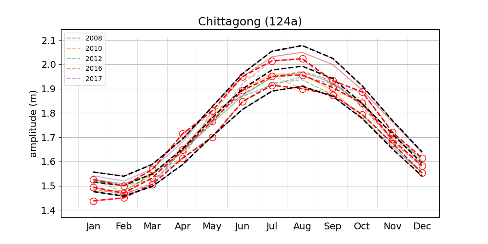
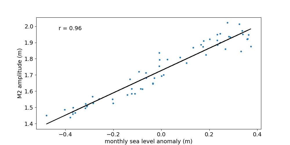
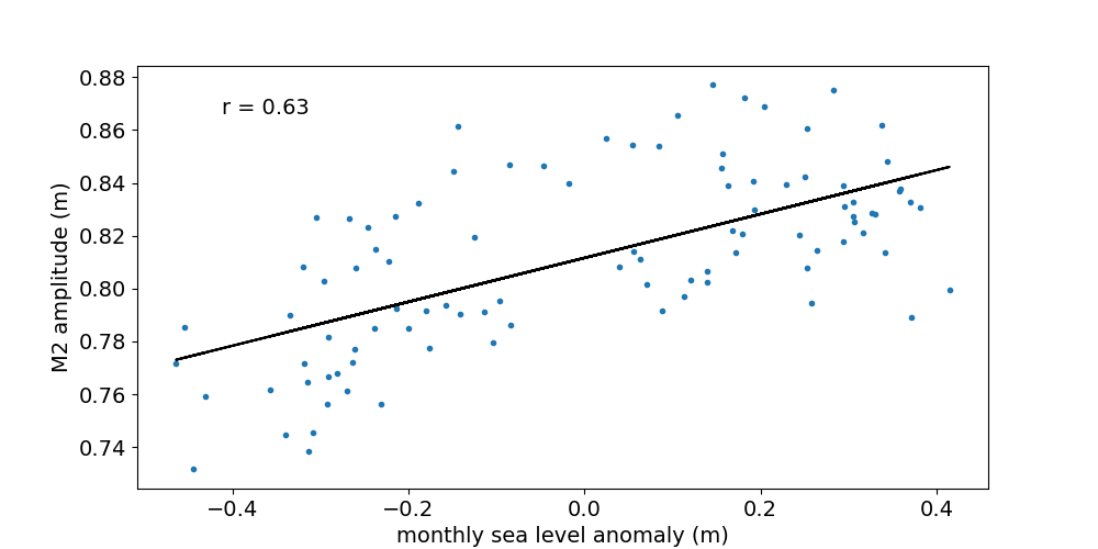
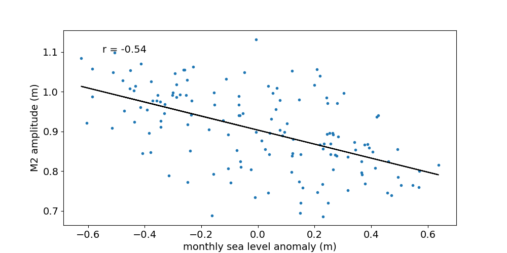
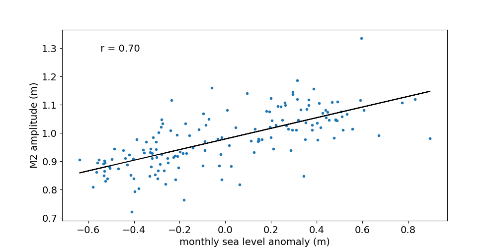
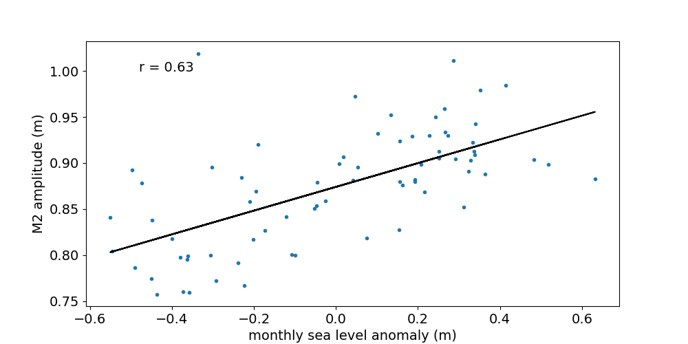
Figure 2 shows the 32-day ("monthly") M2 amplitude as a function of monthly sea level anomaly. The data shown is for the Chittagong station. Plots for the remaining stations can be accessed from the list. The anomaly is measured with respect to the multi-year mean. The individual years chosen for each station are listed e.g in the residual plot table in our previous blog post. The Pearson correlation coefficient between M2 amplitude and monthly sea level anomaly at Chittagong is 0.96. The slope of the fitted line is 0.69 (dimensionless). Two out of six stations (i.e. Cox's Bazaar and Akyab) have a negative correlation coefficient, consistent with the results described above. The magnitude (absolute value) of the correlation coefficient is highest at Chittagong and larger than 0.5 at all stations.

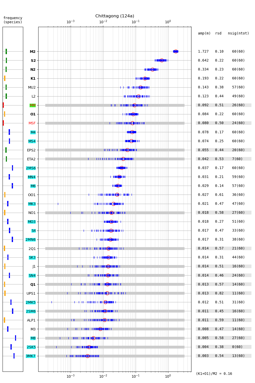
At this point it may be instructive to step back from the focus on seasonal M2 amplitude variation, and make a general comparison between the harmonic analysis results obtained from 32-day intervals and the 366-day intervals described in the companion blog post. Figure 3 shows the amplitudes of tidal constituents computed from 32-day intervals covering multiple years. Compared to the 366-day analysis, fewer tidal constituents are resolved. The largest 4 primary constituents M2, S2, N2, K1 are resolved in the 32-day analysis and the mean amplitude is similar in magnitude to the 366-day analysis. The solar annual constituents SA and the "M2 modulators" \(\alpha_2\) and \(\beta_2\) (H1 and H2 in the notation of Foreman 1977) are obviously unresolved in the 32-day analysis. Here, the constituent with the longest resolved period is the lunar monthly constituent MM, whose mean amplitude is more than three times larger than in the 366-day analysis. Looking at the relative standard deviation, it may be noteworthy that M2 has a small relative deviation in comparison to e.g. the other primary constituents. According to the results shown above, a large part of the relative deviation of M2 is correlated with the monthly mean sea level. At least for S2, the deviations don't seem to be correlated to the monthly mean sea level (not shown).

Figure 3: Amplitudes (m) of tidal constituents at the Chittagong station, computed from 32-day intervals covering all calendar months of the years 2008, 2010, 2012, 2016 and 2017. The horizontal axis of the main panel is logarithmic. The **red circle** shows the mean of amplitudes over all 32-day chunks ("months") considered, independent of whether the signal is significant or not. The value of the mean is listed in the **first column** to the right of the figure. The **second column** shows the relative standard deviation of amplitudes with respect to the mean. The **third column** indicates the number of months in which the signal is significant, i.e. in which it has a signal-to-noise ratio (SNR) > 2 based on the bootstrapped confidence intervals computed by T_Tide (see here for more detailed notes on the software package). The total number of months is shown in brackets. Constituents for which the majority of years yields an non-significant signal are indicated by a **horizontal gray bar**. The constituent's frequency is indicated in the left panel. The horizontal axis of the left panel is a linear function of frequency with convenient units. The constituent species is color-coded as **red** (long period), **orange** (diurnal), **green** (semidiurnal) or **blue** (terdiurnal and shorter periods). The names of primary diurnal and semidiurnal constituents are printed in **bold fonts**. Shallow water constituents are **labelled cyan**. Note that shallow water constituents may be masking main constituents, in which case the label is not coloured in cyan. Long-period constituents are written in **red fonts**. The long-period constituents usually dominated by meteorological phenomena, and explicitly labelled as such in table A.1. of Parker (2007), are **labelled green**. Note that table 3.2 in Parker (2007) lists MSF and MF as usually dominated by meteorological phenomena, and does not list MSM. For further comparison, table 3.2 of Parker (2007) lists the 37 constituents that are typically included in a harmonic analysis at NOAA (see also here for an example. For a comparison to amplitudes computed from a 366 day interval covering 2008, see here.

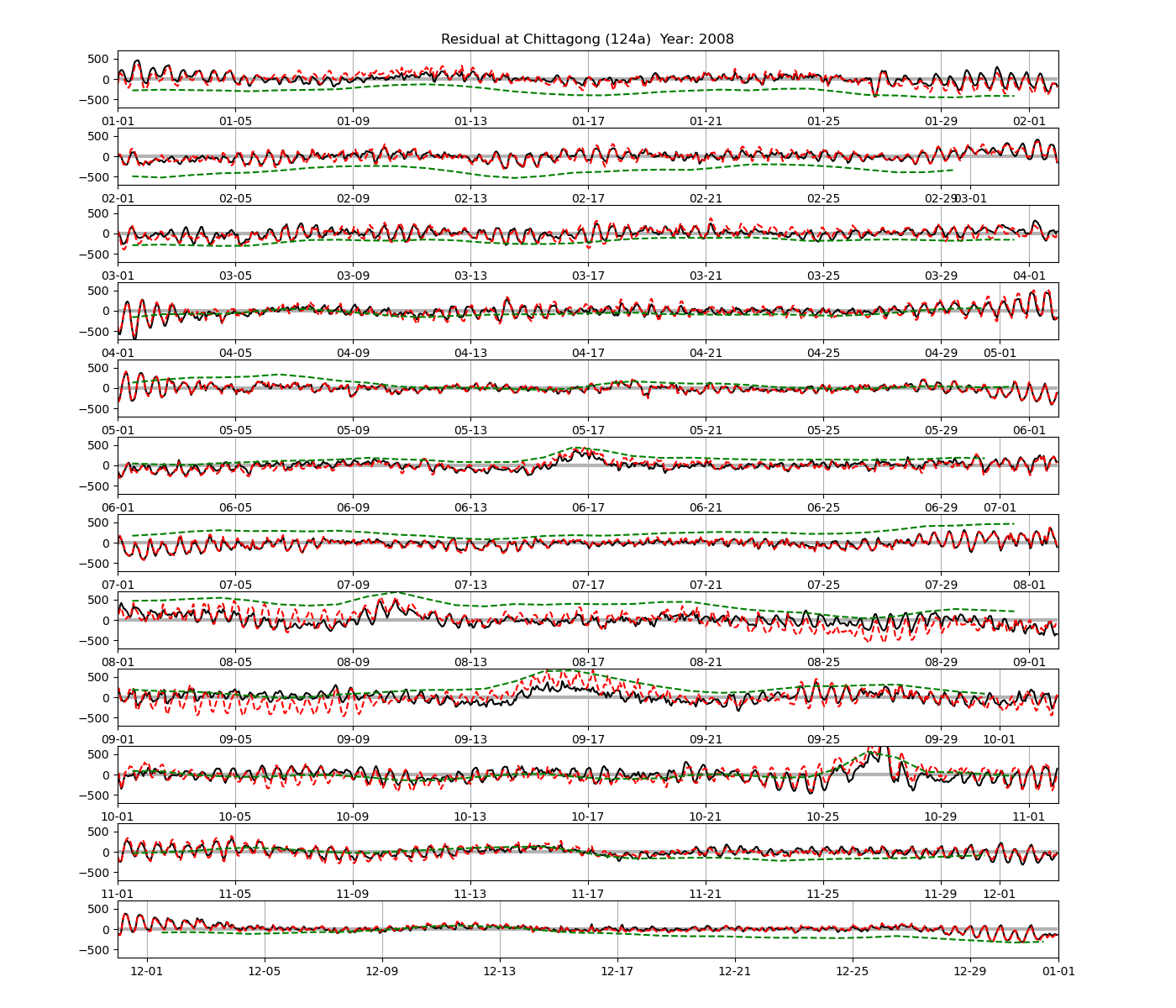
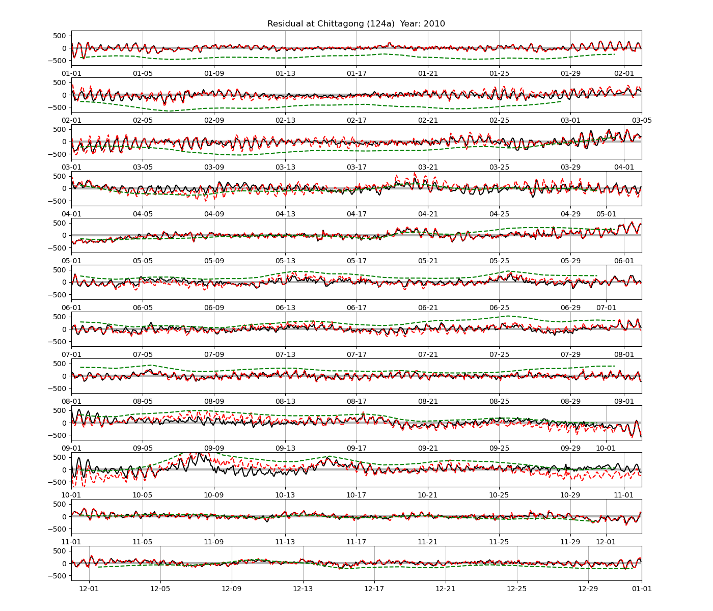
As a further comparison to 366-day harmonic analysis, Figure 4 shows the residual sea level at the Chittagong station for predictions calculated from harmonic analysis of 32-day segments. In comparison with the residual computed from the 366-day analysis, the semidiurnal oscillations seem to be lower in some segments of the time series, and there seems to be a tendency for the residual to be larger at the beginning and end of the 32-day segment.

5 Summary and discussion

We quantify the seasonal variation of M2 amplitude at 6 tide gauges in the north-eastern Bay of Bengal. The data was obtained in preprocessed form from UHSLC and/or other third parties (see acknowledgements6 ). Harmonic analysis was performed with T_Tide, a popular harmonic analysis toolbox.

Following Müller et al. (2014), we use two methods to quantify the seasonal variation of M2 amplitude. The first method uses 32-day sections of water level time series and computes the M2 amplitude for each section. The second method uses 366-day sections and computes the harmonic constants of M2 and two additional satellites, which induce an annual variation in the composite signal (e.g. Corkan, 1934).

At 4 out of 6 stations, the M2 amplitude is low in summer and high in winter. The remaining two stations are located at the east coast of the Bay of Bengal where the shelf slope is steeper than adjacent to and west of the GBM delta. The remaining two stations show a reverse pattern with higher (lower) amplitudes in summer (winter). The two methods largely produce similar overall seasonal cycles of the multi-year mean seasonal cycle.

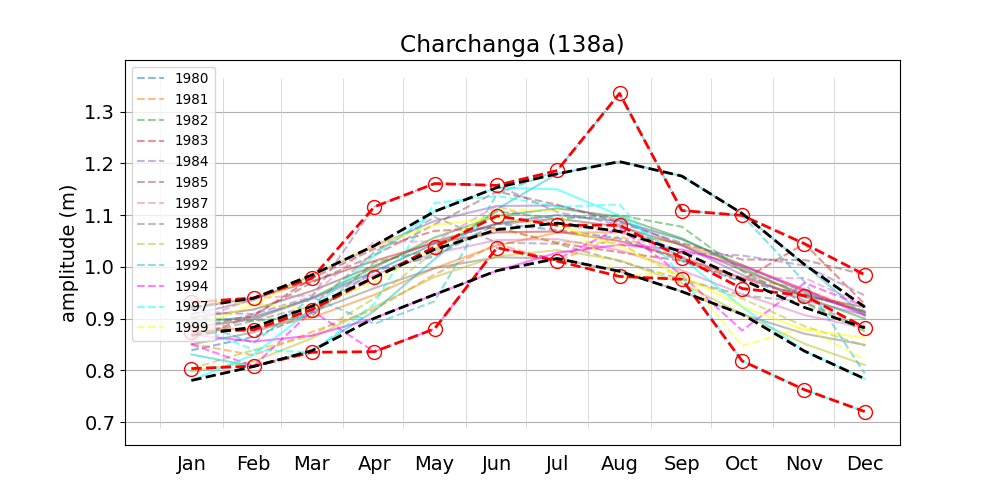
The results mostly agree with those of Tazkia et al. (2017), who use method 1 (but with a sliding window of 2 months) to find absolute seasonal differences between M2 amplitudes of 8 cm at Hiron Point and 21cm at Charchanga.

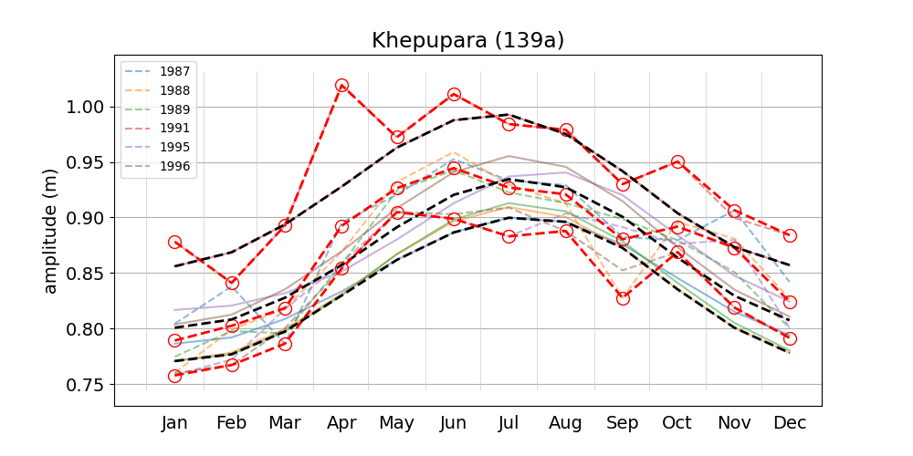
Müller et al. (2014) point out a drawback of method 2, i.e. that it implies sinusoidal amplitude variations based on the fundamentals of harmonic analysis. They show two examples for which the use of constituents \(\alpha_2\) and \(\beta_2\) yields unsatisfactory results, i.e. in the case where the annual cycle of the amplitude is not approximately sinusoidal. Looking at Figure 2 of Tazkia et al. (2017), and e.g. our Figure 5 (Hiron Point), Figure 8 (Khepupara) or Figure 9 (Akyab), this issue may indeed be problematic in the region under consideration. We speculate that this may be the reason why Tazkia et al. (2017) opted for method 1. However, for the purpose of model calibration, there is arguably value in determining true harmonic constants for the main constituents, which are by definition constant in time. Such an analysis should arguably be done with segments of (at least) annual length to average out the seasonal variation, but will inevitable also produce relatively large seasonal "meteorological modulators". It seems important to distinguish these from "true" harmonic constants associated with gravitational forces induced by astronomic objects.

6 Acknowledgements

We thank UHSLC, the director of Meteorology CIVAIR at the SEEB International Airport of the Sultanate of Oman, and the Bangladesh Inland Water Transport Authority (BIWTA) for providing data. We thank the authors of IOS Tidal Package and T_Tide for providing their software. Figures in this blog post have been prepared with matplotlib (Hunter, 2007) and NumPy (Harris et al., 2020). T_Tide has been slightly modified to run in GNU Octave (Eaton et al., 2020).

7 Appendix A

8 Appendix B

The classical method of amplitude modulation in signal transmission and processing may be applied to \eqref{eq:eq1} under certain conditions. Sufficient conditions are that (1) all \(\phi_i\) vanish and (2) that \(a_2=a_3\). Denoting the common phase lag as \(\phi\) and

\begin{gather*} f_c := f_1 = 2f_{L}\\ f_m := f_c - f_2 = f_{SA} \\ a_c := a_1 \\ a_m := a_2 = a_3 \end{gather*}

where \(f_c\) and \(a_c\) denote the carrier frequency and amplitude, and \(f_m\) and \(a_m\) denote the modulation frequency and amplitude, Eq. \eqref{eq:eq1} reads

\begin{gather} \zeta_{comp}(t) = a_c\cos{(2\pi f_ct)} \notag \\ + a_m\left\{ \cos{\left[2\pi (f_c-f_m)t\right]} + \cos{\left[2\pi (f_c+f_m)t\right]} \right\} \notag \\ = a_c\cos{(2\pi f_ct)} \notag \\ + 2a_m \cos{\left(2\pi f_ct\right)} \cos{\left(2\pi f_mt\right)} \notag \\ = \cos{(2\pi f_ct)}\left[ a_c + 2a_m\cos{\left(2\pi f_mt\right)} \right] \notag \\ = A(f_m,t)\cos{(2\pi f_ct)},\label{eq:eq2} \end{gather}

where we have used that

\begin{gather*} \cos{a}\cos{b} = 0.5\left[\cos{(a+b)} + \cos{(a-b)}\right]. \end{gather*}

Importantly, the term \(A(f_m,t)\) in Eq. \eqref{eq:eq2} is independent of the carrier frequency \(f_c\). Under the conditions imposed above, the amplitude of the modulated M2 signal varies with annual frequency \(f_{SA}\).

The question arises whether the conditions imposed above are not only sufficient, but also necessary to obtain the general form \(A(f_m,t)\cos{(2\pi f_ct)}\). Initial attempts by the author to reproduce Eq. (22) of Müller et al. (2014), where \(a_2\), \(a_3\) and all three \(\phi_i\) differ, were unsuccessful, and we speculate that they may contain an error. Here we simply estimate the amplitude by numerical methods.

References

Caldwell, P.C., Merrifield, M.A., Thompson, P.R., 2015: Sea level measured by tide gauges from global oceans — the Joint Archive for Sea Level holdings (NCEI Accession 0019568), Version 5.5, NOAA National Centers for Environmental Information, Dataset, doi:10.7289/V5V40S7W.
Caldwell, P.C., 2015: Hourly Sea Level Data Processing and Quality Control Software: Version for Linux Operating Systems. SLP64 User Manual
Corkan, R.H., 1934: An annual perturbation in the range of tide.
Dube, S.K., Rao, A.D., Sinha, P.C., Murty, T.S., 1997: Storm surge in the Bay of Bengal and Arabian Sea the problem and its prediction.
Eaton J.W., Bateman D., Hauberg S., Wehbring R., 2020: GNU Octave version 6.1.0 manual: a high-level interactive language for numerical computations.
Foreman M.G.G, 1977: Manual for Tidal Heights Analysis and Prediction. Pacific Marine Science Report 77-10, Institute of Ocean Sciences, Patricia Bay, Sidney, B.C., 58 pp. (2004 revision)
Godin, G., Taylor, J., 1973: A simple method for the prediction of the time and height of high and low water.
Godin, G., 1972: The Analysis of Tides.
Harris, C.R., Millman, K.J., van der Walt, S.J., others, 2020: Array programming with NumPy.
Hunter, J.D., 2007: Matplotlib: A 2D Graphics Environment.
Intergovernmental Oceanographic Commission, 1992: Joint IAPSO-IOC Workshop on Sea level measurements and quality control, Paris, 12-13 October 1992. (ed. N.E.Spencer)
Müller, M., Cherniawsky, J.Y., Foreman, M.G., von Storch J.S., 2014: Seasonal variation of the M2 tide.
Parker, B.B., 2007: Tidal analysis and prediction. NOAA Special Publication NOS CO-OPS 3, U.S. Department of Commerce, 378 pp.
Pawlowicz, R., Beardsley, B., Lentz, S., 2002: Classical tidal harmonic analysis including error estimates in MATLAB using T_TIDE.
Tazkia, A.R., Krien, Y., Durand, F., Testut, L., Islam, A.S., Papa, F., Bertin, X., 2017: Seasonal modulation of M2 tide in the Northern Bay of Bengal.

Harmonic analysis of tide gauge data in the north-eastern Bay of Bengal: Seasonal variation of M2 amplitude

1 Abstract