Harmonic analysis of tide gauge data in the north-eastern Bay of Bengal: Amplitudes and residuals for 366 day intervals
Riha, S.1 Abstract
We conduct harmonic analysis of water level time series measured at 6 tide gauges in the north-eastern Bay of Bengal. Results include listings of harmonic amplitudes and residual time series for selected tide gauge stations. The analysis is limited to time series intervals of 366 days. The preprocessed water level data was obtained from the Joint Archive for Sea Level maintained by the University of Hawaii Sea Level Center (UHSLC). The primary motivation of this blog post is to re-compute and publish harmonic constants of selected UHSLC data, given that UHSLC does not seem to publish the harmonic constants computed for their analysis. We raise some questions relating to the use and the interpretation of additional constituents to express the seasonal, meteorologically induced modulation of the lunar semidiurnal constituent M2. The author has no prior experience with harmonic analysis. Corrections and comments via E-mail are appreciated.
2 Introduction
Tide gauge data is crucial for storm surge modelling. Variations of water level are produced by gravitational forces of astronomical objects and geophysical events. Harmonic analysis is commonly used to separate out periodic signals at tidal frequencies from more transient or irregularly occurring events. The calibration of hydrodynamic models for water level prediction relies heavily on the analysis of tides. In particular, parametrizations for frictional effects used in barotropic storm surge models can be validated against tide predictions computed from harmonic analysis.
Storm surges caused by tropical cyclones are a serious hazard, for example along the coasts of India, Bangladesh, Myanmar and Sri Lanka (Dube et al., 1997). Bangladesh is particularly exposed due to
- shallow coastal water adjacent to the Ganges-Brahmaputra-Meghna (GBM) Delta
- convergence of the Bay to the north
- high astronomical tides
Tazkia et al. (2017) described the seasonal changes of amplitude of the semi-diurnal lunar tide adjacent to the GBM delta. They use a barotropic model to mimic the effect of apparently mostly baroclinically induced seasonal sea level variations onto tidal amplitudes. Seasonal sea level variations in the north-eastern Bay of Bengal are forced by a combination of local and remote mechanisms. Local effects include wind stress, freshwater discharge and atmospheric pressure waves associated with the monsoon. Remote effects include Kelvin waves excited in the equatorial ocean and propagating northward along the east coast into the Bay of Bengal, where some fraction of the energy propagates westward as Rossby waves into the interior Bay. Han and Webster (2002) use a 4.5-layer reduced-gravity model and identify equatorial wind variability as the dominant driver for interannual variability of sea level in the north-eastern region of the Bay.
The strong seasonal signal induced by meteorological phenomena is interesting from the perspective of tidal analysis. Seasonal sea level cycles with a period of one year directly affect the solar annual tidal constituent. Furthermore, the meteorologically forced seasonal modulation of the principle semidiurnal constituent M2 as described e.g. by Tazkia et al. (2017), likely produces spectral peaks in the vicinity of M2, separated from M2 by a frequency of about 1/y. The practice of defining a new "meteorological constituent" that modulates M2 with annual frequency, goes back at least to Corkan (1934). Müller et al. (2014) note that the resulting annual constituents are sometimes referred to as \(\alpha_2\) and \(\beta_2\) in the literature. In section 5 we discuss slight differences between \(\alpha_2\) and \(\beta_2\) and the constituents proposed by Corkan (1934), which may be confusing to beginners of harmonic analysis. Quantitatively, this difference may be irrelevant for the purpose of this study. In Appendix B we argue that Eq. 22 of Müller et al. (2014) may contain an error.
Here we try to prepare for further studies and conduct harmonic analysis of water level at 6 stations in the north-eastern Bay of Bengal. Results include harmonic amplitudes and residual time series computed from 366 day intervals. Analysis of shorter intervals, as e.g. performed by
Tazkia et al. (2017), is deferred to future work. The predictive value of harmonic constants in the region of interest is questionable, given the strong influence of meteorology on the water level. The main motivation for computing these constants is for calibration of numerical models. We use preprocessed hourly and daily water level data from the Joint Archive for Sea Level (JASL, see
Caldwell et al. 2015), maintained by the University of Hawaii Sea Level Center (UHSLC) 
3 Methods
3.1 Observations and data
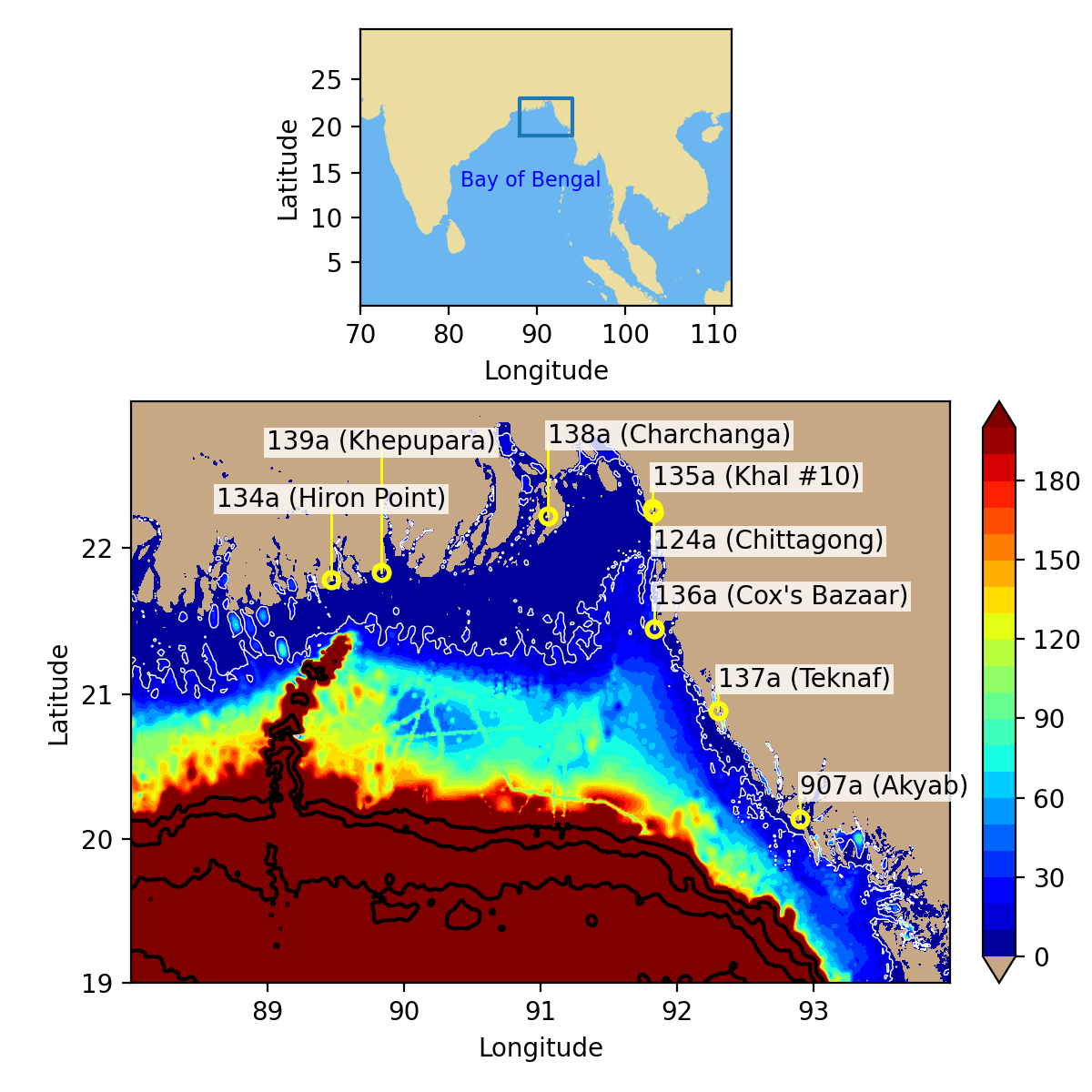
Figure 1 shows a map of the head bay of the Bay of Bengal and the location of 8 tide gauges. Here we refer to this region simply as north-eastern Bay of Bengal. UHSLC maintains an archive of research-quality water level data with hourly and daily resolution, containing (among many others) the depicted gauges. Note that the locations of stations "Khal #10" and Chattogram (formerly known as Chittagong) are barely distinguishable on the map. Khal #10 seems to be located slightly upriver of the Chittagong station (detail not shown). Note also that the location coordinate metadata for the tide gauge in Cox's Bazaar may be incorrect. A detailed description of the bathymetry around individual stations will be presented in a future study along with results from numerical modelling.
The tide gauge data is preprocessed by UHSLC (Caldwell et al., 2015) and/or possibly other third parties. IOC (1992) describe the standardized data processing and quality assurance methodology followed to produce the Research Quality dataset archived by the NOAA National Centers for Environmental Information as the Joint Archive for Sea Level (JASL, see Caldwell et al. 2015). The quality assessment policy (FTP link) states that assessment is mostly based on residuals (observed data minus predicted tides) of hourly data. IOC (1992) state that the hourly data is computed from the high-frequency data delivered by the instrument via a three-point Hanning filter. In at least some of the station metadata described below, it is explicitly mentioned that the filter is centered on the hour. IOC (1992) further state that the filter was chosen to minimize aliasing from subsampling and to minimize the attenuation of the tides. The archive also contains daily time series. Caldwell (2015) describes the two-step tidal filtering procedure for computation of the daily values. In a first step, dominant diurnal and semi-diurnal tidal components are removed from the quality controlled hourly values. Secondly, a 119-point convolution filter is applied to remove the remaining high frequency energy and to prevent aliasing. In this post we mostly use hourly data, but also show filtered ("de-tided") daily data in the plots of the monthly mean sea levels and the residual time series.
In this blog post we present results from harmonic analysis and discrete Fourier transforms, and point out that we do not assess the sensitivity of our results to the choice of any low-pass filters used to produce the hourly data. In particular, any energy contained in high frequencies of the physical (continuous) quantities, which may not have been filtered, will project onto discretized lower frequencies via aliasing.
Each station (i.e. time series) is accompanied by an individual quality assessment report issued by UHSLC, containing information such as missing data, notes on the reference level, spurious fluctuations, etc. (see e.g. here for examples for the Indian Ocean, but note that this is an FTP link which your web browser may refuse to follow 
- a Completeness Index ("CI") indicating the percentage of hours with available data, which may include replacements of gaps of less than 25 hours by prediction data
- a list of gaps longer than a day. These are not patched with prediction data, and instead are filled with a missing data flag. The format of the list is e.g. "44-45,325-330,352-353" referring to 3 gaps, the first of which starts at some (unspecified) hour on year-day number 44 and ends at some hour on year-day number 45. We found that the exact hours can most easily be retrieved by searching for the missing data flag in a human-readable format of the data files (e.g. the comma-separated-value format distributed by UHSLC).
- a summary of days with consecutive missing or obviously wrong data in a time span longer than 6, but less than 25 hours that have been replaced with prediction data, with hours in parentheses.
- a summary of days with questionable fluctuations in the residual series. Fluctuations within the residuals are considered significant and are noted if they are greater than 25 cm. This policy has changed slightly as of October 1992: only suspicious fluctuations due to obvious instrumentation problems are noted. Minor timing drifts are no longer included in the list of questionable days.
For our purposes we pick out years with a CI of 100% and with as few questionable fluctuations as possible. We do not consider the stations Khal #10 and Teknaf. Some time series contain replaced gaps. This implies that our harmonic analysis is based on a previous harmonic analysis performed by UHSLC, and hence could be described as somewhat circular or iterative. One motivation to repeat the analysis is simply that UHSLC do not seem to publish their computed harmonic constants, perhaps because they are merely a by-product of their quality control procedure. Also note that one particular advantage of harmonic analysis based on least squares over discrete Fourier analysis is the ability to handle data gaps and irregularly spaced data. Since there are no data gaps in our (already patched) time series, and the interval is constant, the question arises what further advantages harmonic analysis has. This is issue not further discussed in this blog post and the reader is referred to the literature (e.g. Parker, 2007, their section 3.4.5).
3.2 Harmonic analysis method and software packages
The general method of harmonic analysis based on the least squares solution is described e.g. in Foreman and Henry (1989).
Given an observed time series \(\zeta(t)\) of water level above a reference datum, one may define a predicted water level as
where \(n\) is the number of tidal constituents and \(\omega_i\) the constituent's angular velocity. The objective is to find harmonic constants, i.e. amplitude \(a_i\) and phase \(\phi_i\) for each constituent (and the constant \(Z_0\)), such that the residual time series
is minimal in a least-square sense. Amplitudes and phases may be modified by nodal corrections.
We use the SLP64 


The notes on IOS Tidal Package and T_Tide describe some differences between the software packages in more detail. Here we only point out that there are slight differences in the predicted water levels, and hence the residual time-series. First, the packages apply nodal modulation corrections differently in their tidal predictions. Secondly, T_Tide is able to compute confidence intervals or signal-to-noise ratios for each harmonic constant (Pawlowicz et al., 2002). In its default configuration, T_Tide version v1.3_beta will include only significant constituents in the prediction of the water level, and hence also in the computation of the residual water level. More details are given in the companion blog post.
For this blog post we simply adopt the default parameters of the t_tide.m routine in T_Tide version v1.3_beta. At this stage we do not attempt to justify this choice in the context of this study. Instead, the results presented here serve to gain intuition about the meaning and usefulness of these confidence intervals. Hence the figures of residual time series below will show two residuals throughout this blog post, where one is computed with IOS Tidal Package using all constituents, and the other is computed with T_Tide using only significant constituents. We interpret a constituent as statistically significant if its harmonic constants have an SNR>2, following the default configuration of T_Tide.
3.3 Data processing
In applying the harmonic analysis method to the UHSLC data we loosely follow the steps outlined in chapter 4.5 of Parker (2007) and the manual of SLP64. We analyze time series of 366 consecutive days, as outlined in the manual of SLP64. For non-leap years, we choose the 365 days of the calendar year, and add the first day of the subsequent year. According to the constituent sorting strategy of Foreman (1977), the number of resolvable constituents with this length is 67, i.e. 44 main constituents (excluding the constant constituent Z0) and 24 shallow-water constituents. Note that the astronomical constituent Γ2 listed in Table 1 of the companion blog post is not resolvable, since a time series of about 472 days would be necessary to separate it from H1 (α2) (Foreman, 1977, their Table 3)..
As an example for the data processing, consider the year 2008. This is a leap year and hourly observations from 2008/1/1 00:00 UTC to 2008/31/12 23:00 UTC yield 366*24=8784 observations. Both IOS Tidal Package (provided with SLP64) and T_Tide will clip the last observation to obtain an odd number of observations (Foreman, 1977, their section 2.2.1).
4 Results
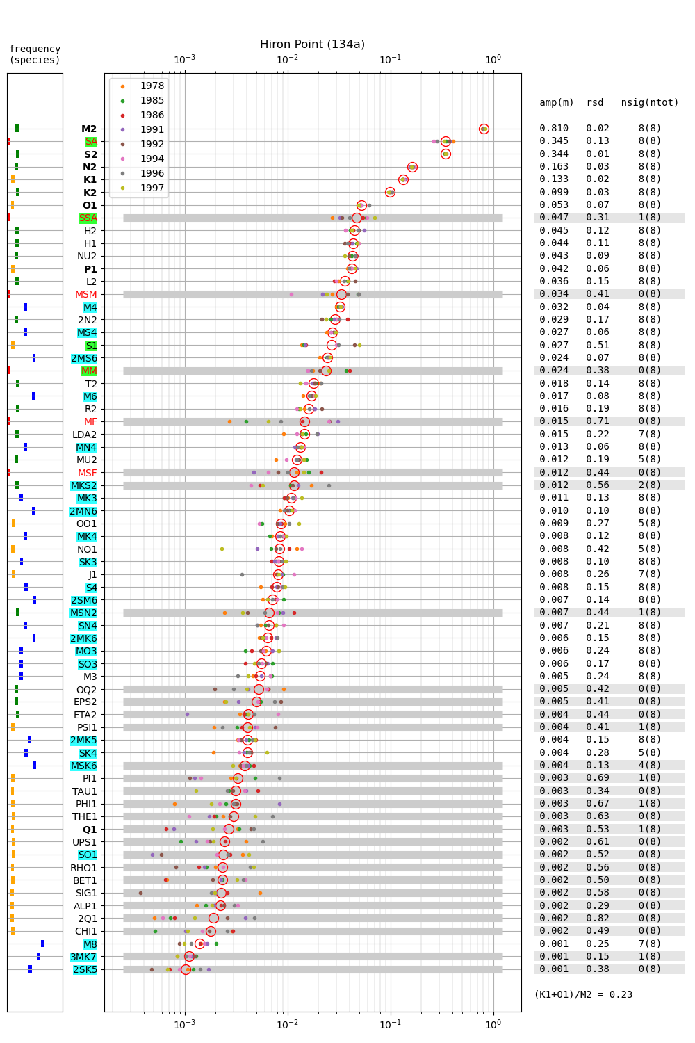
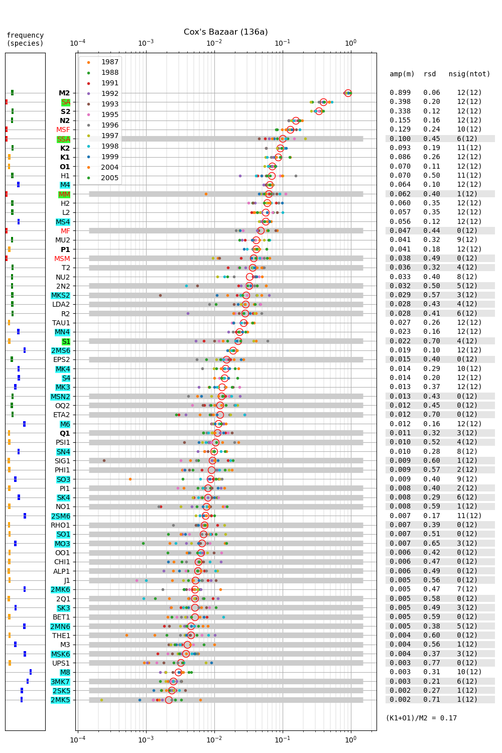
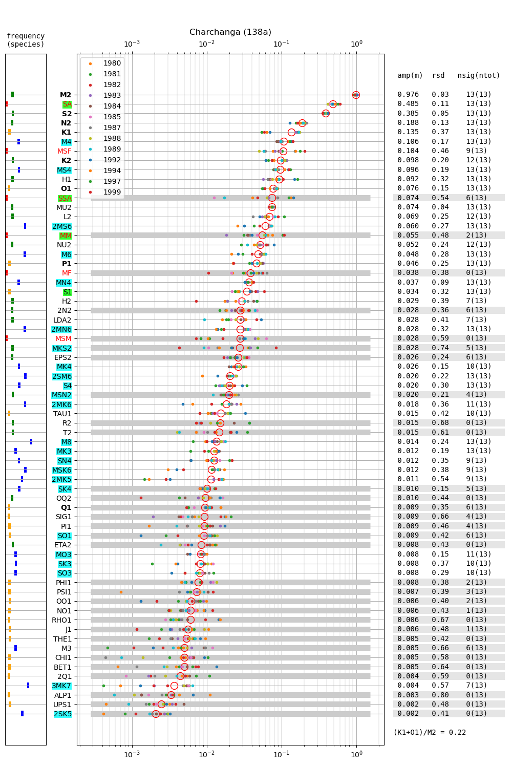
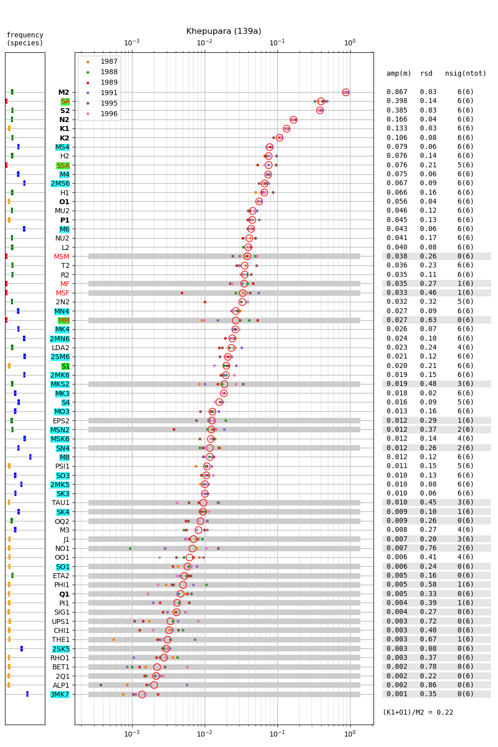
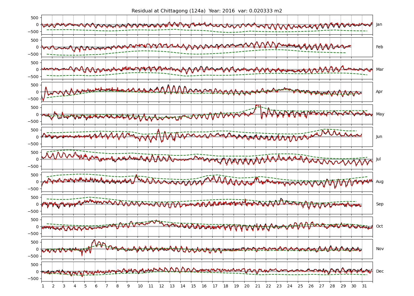
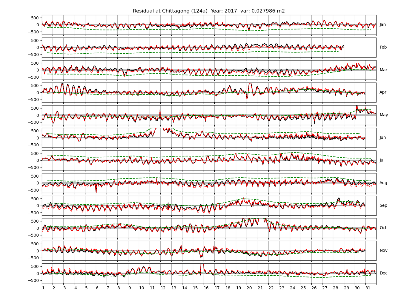
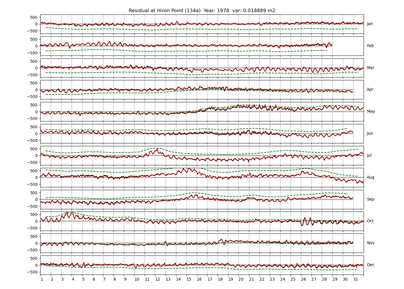
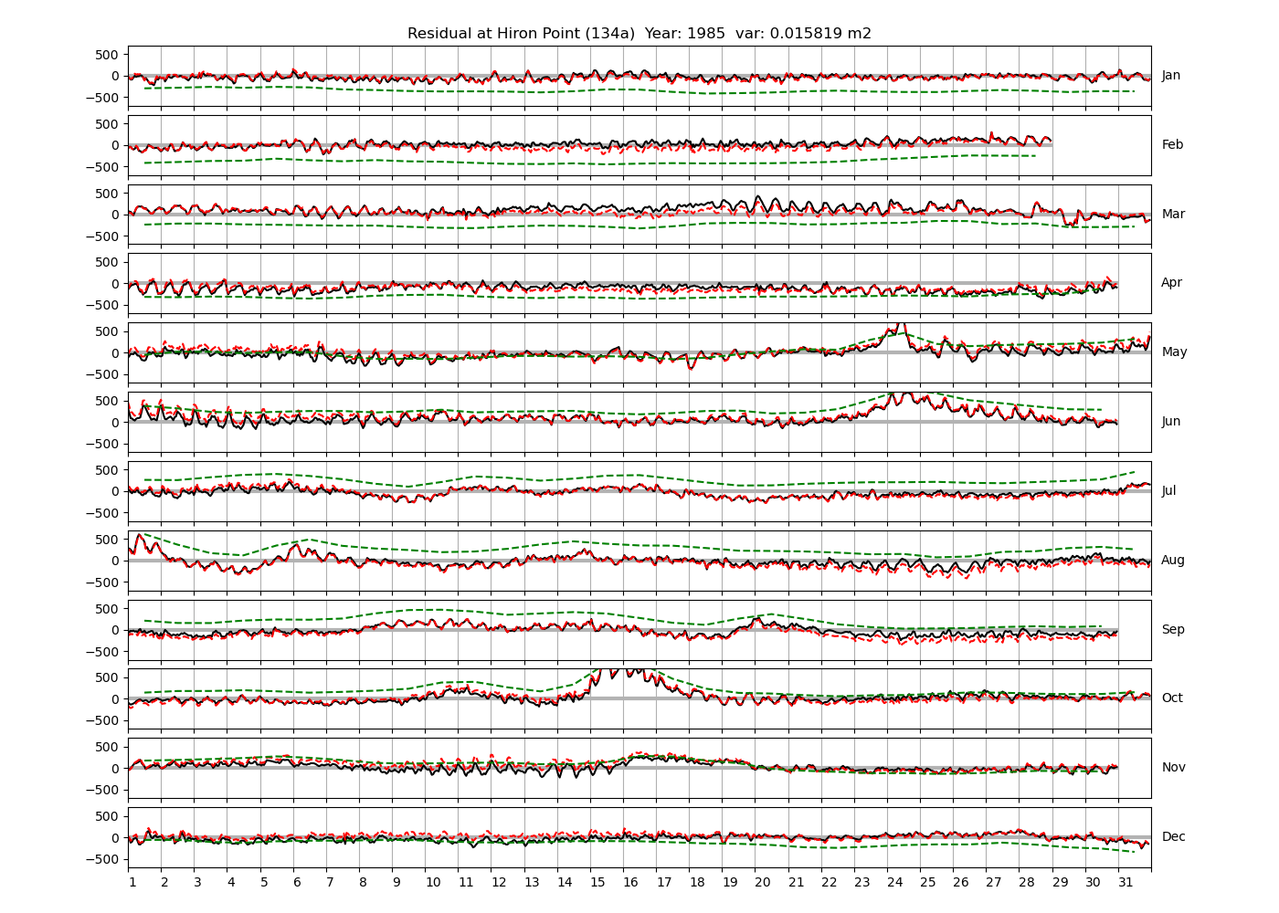
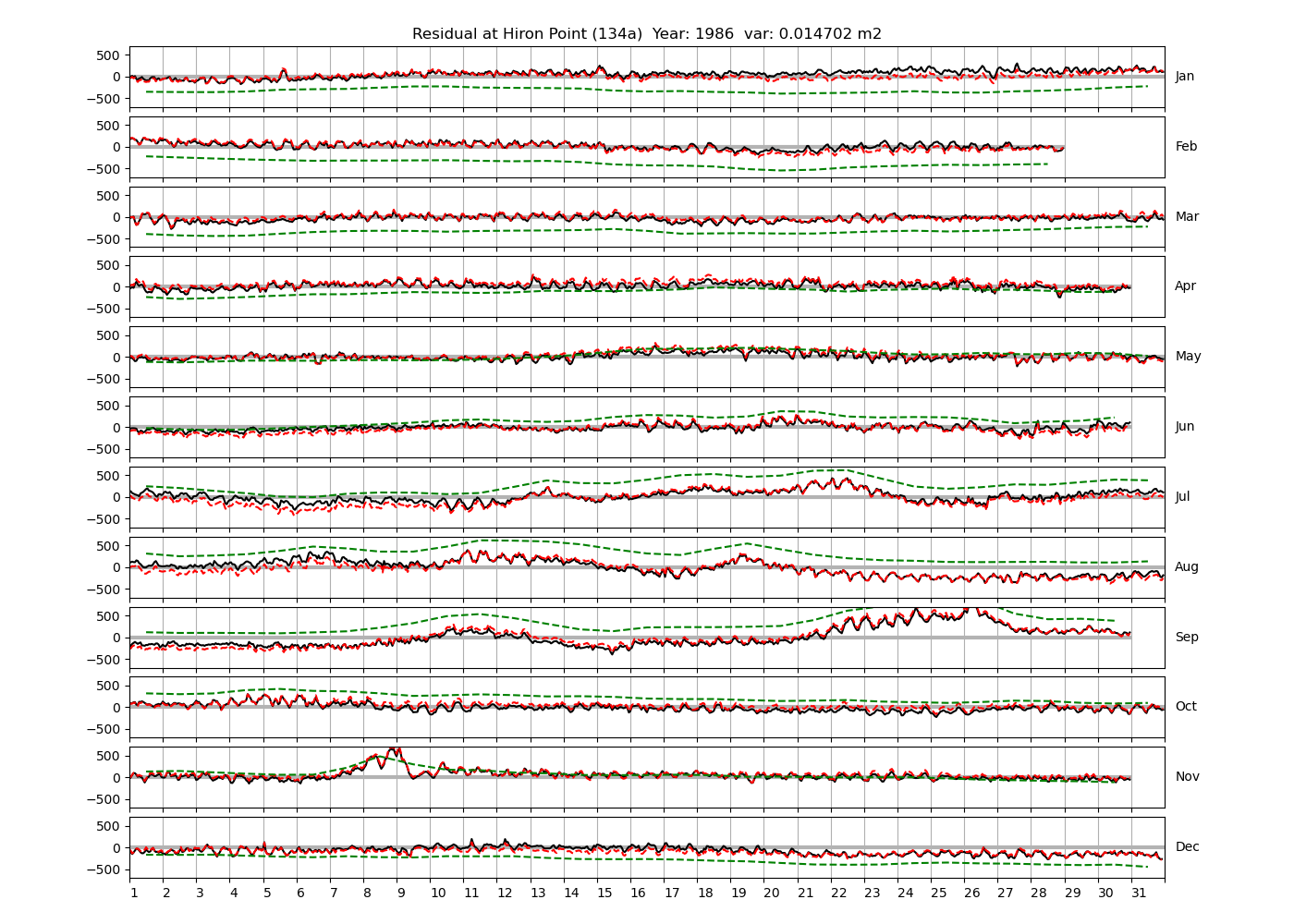
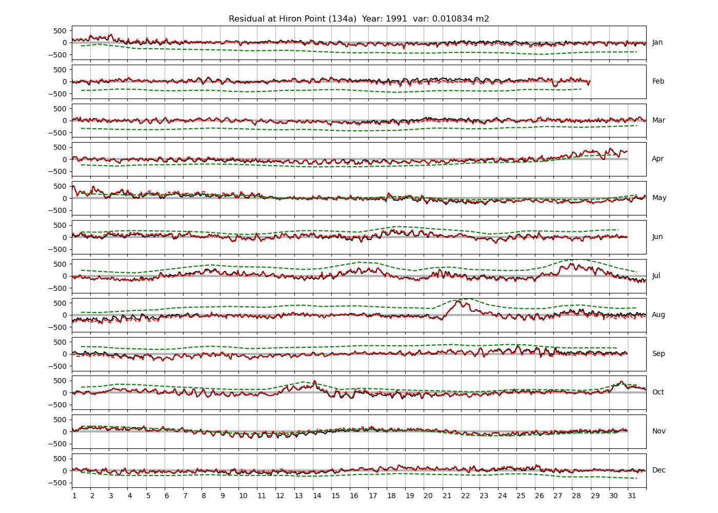
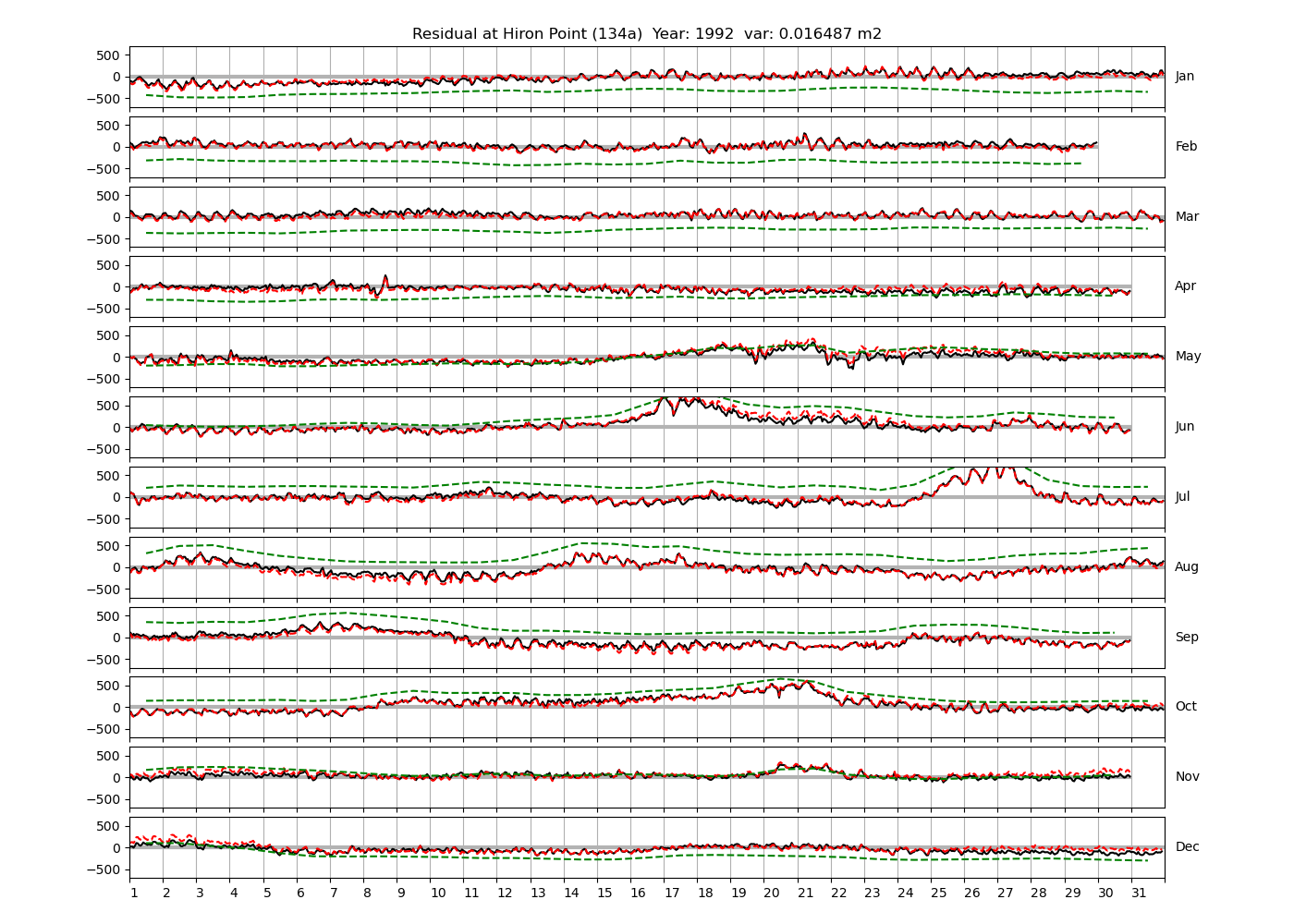
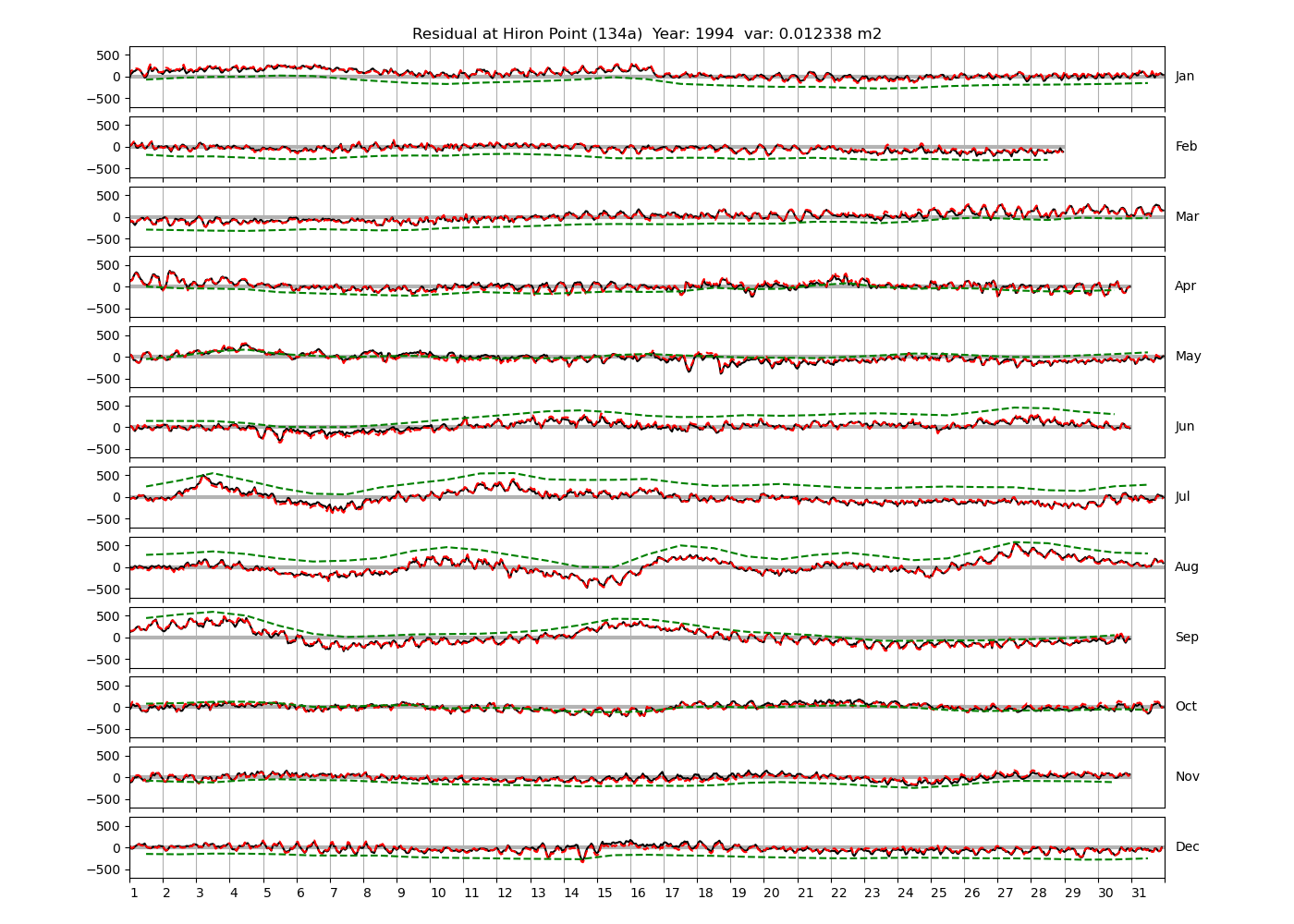
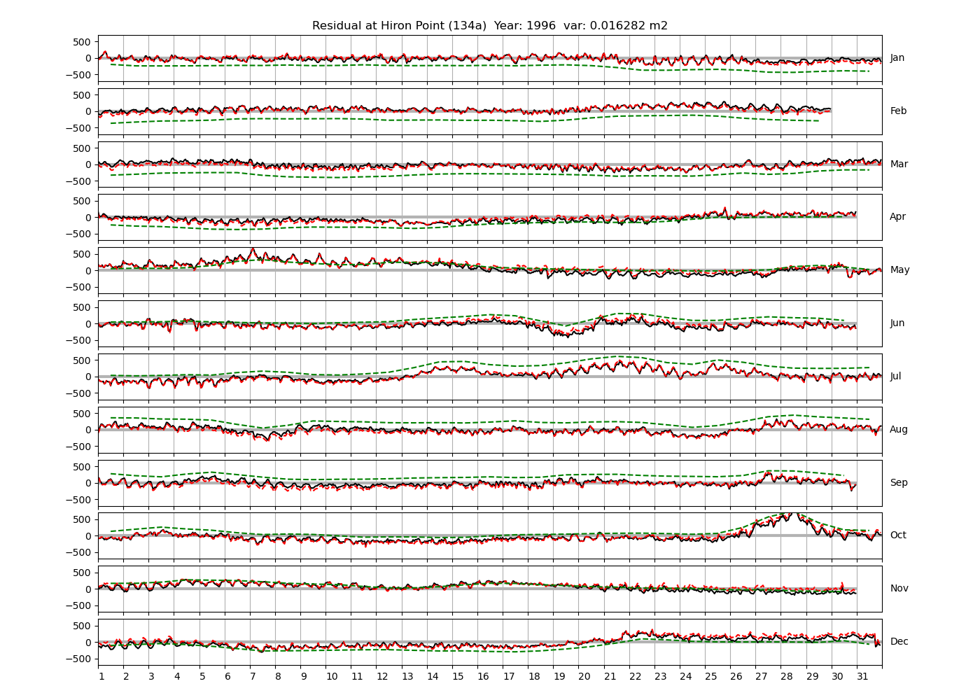
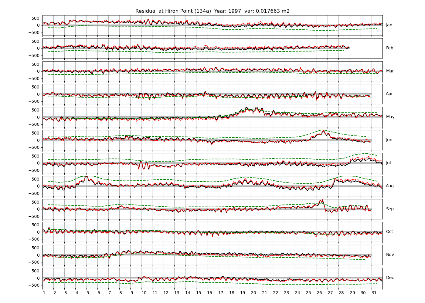
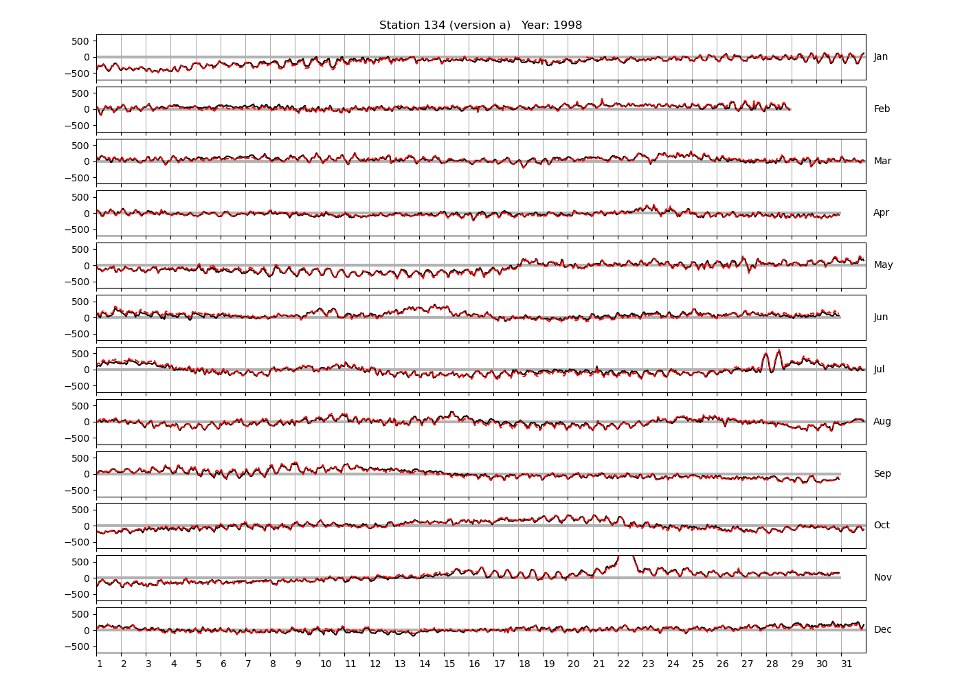
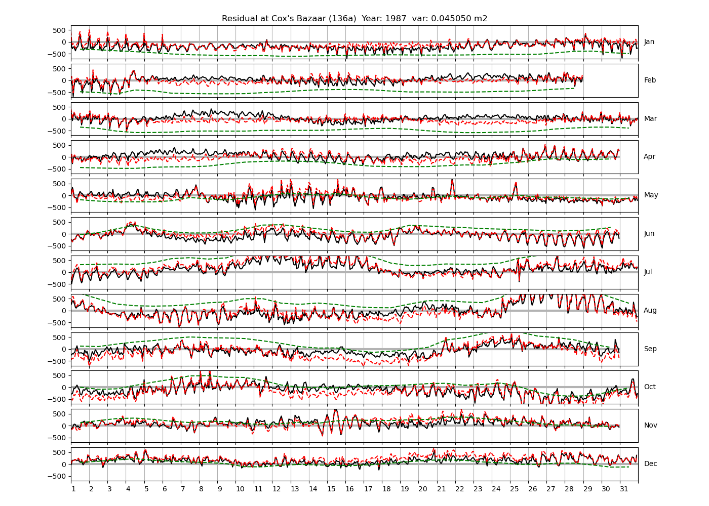
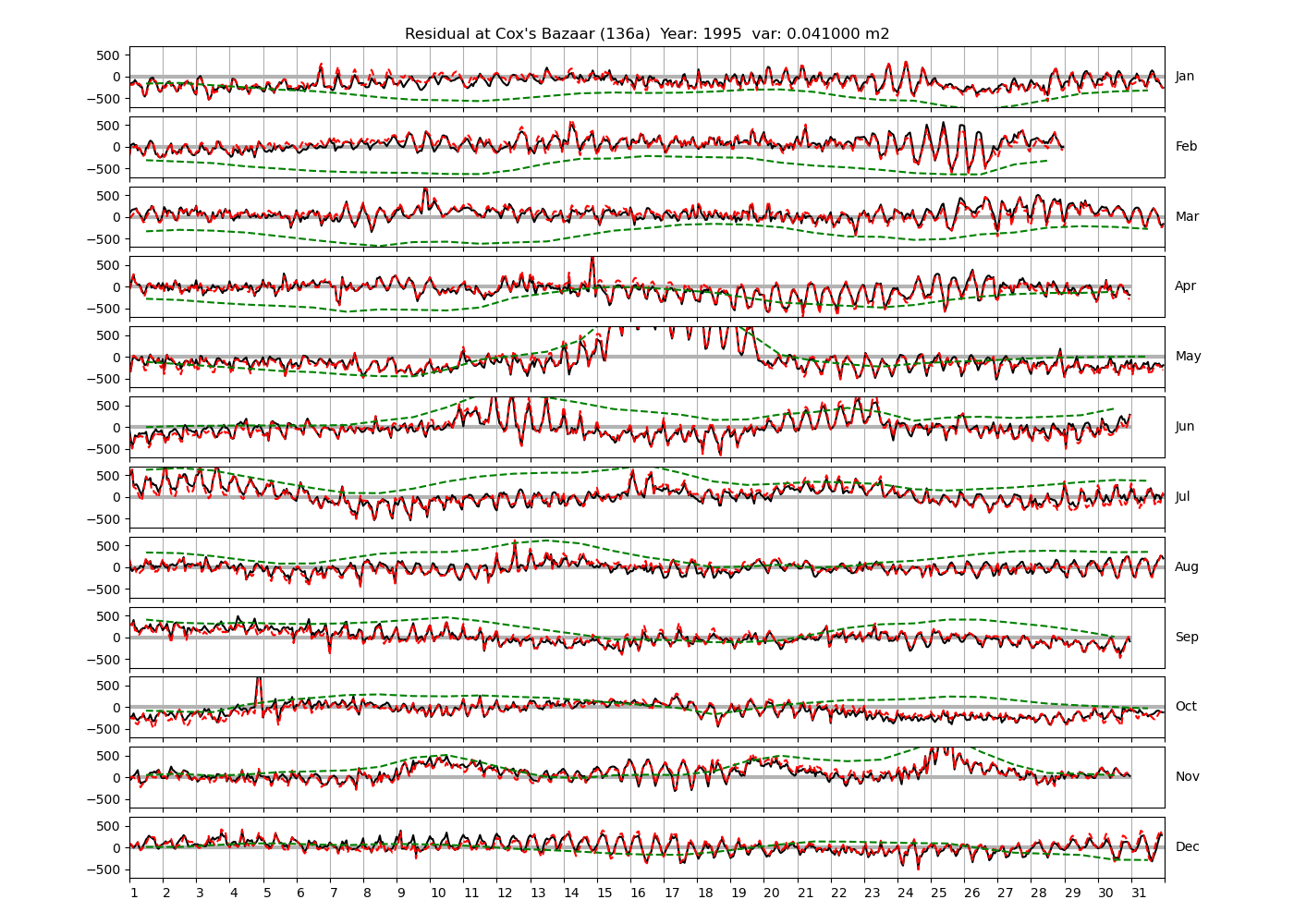
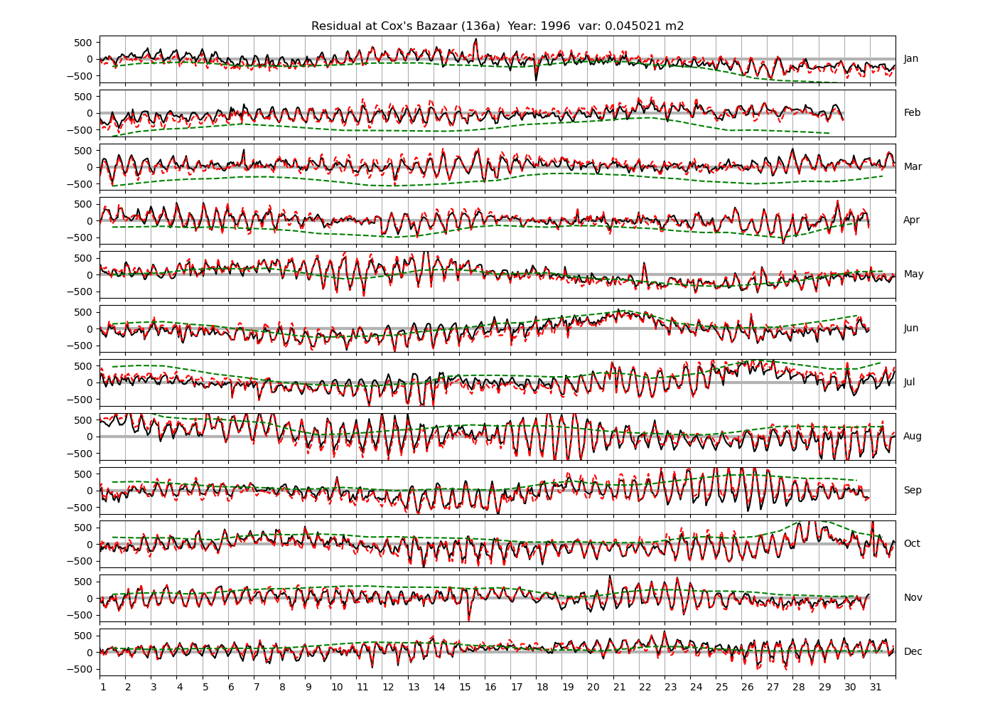
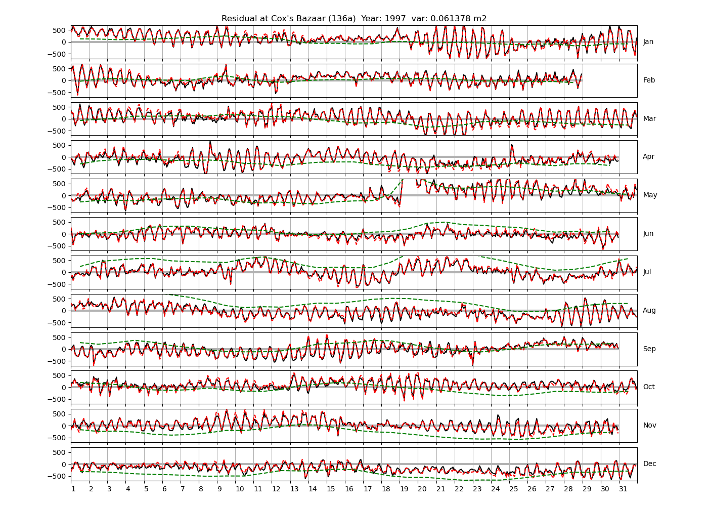
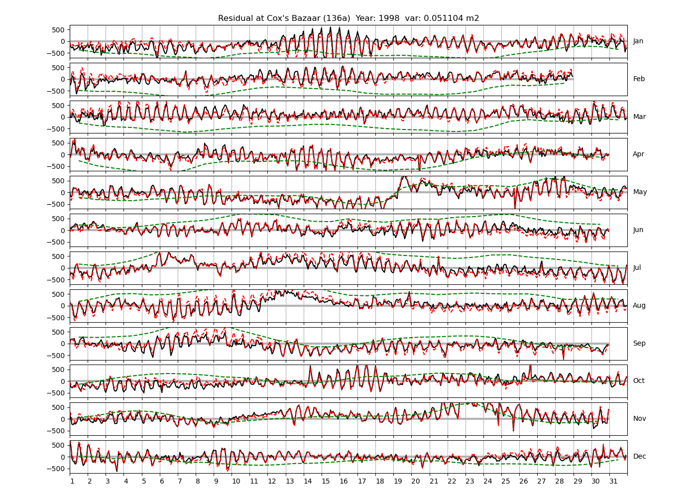
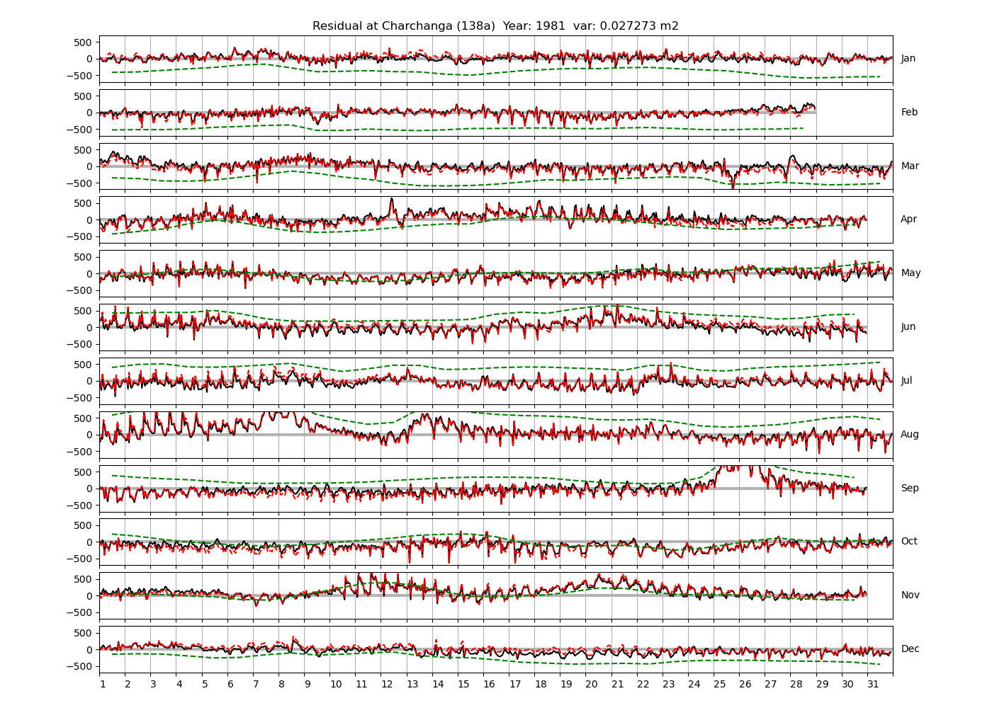
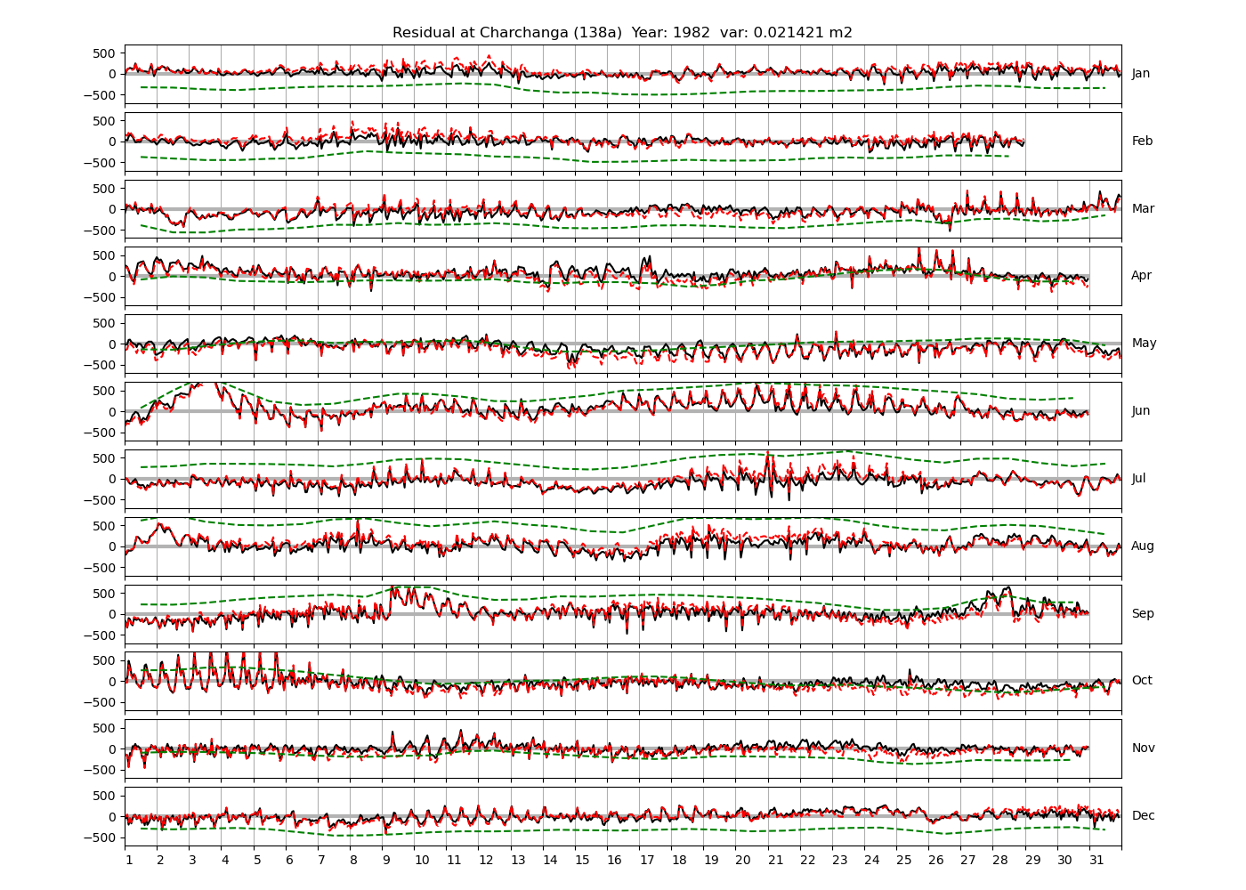
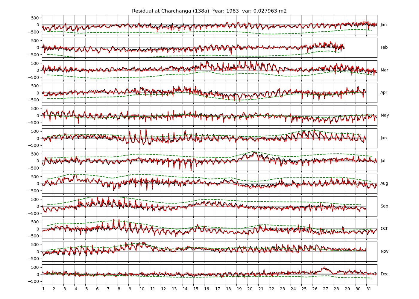
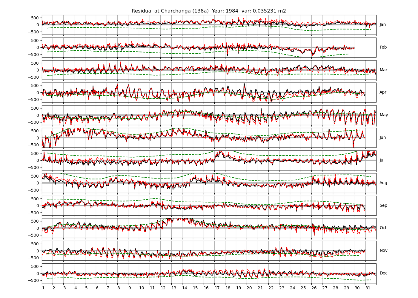
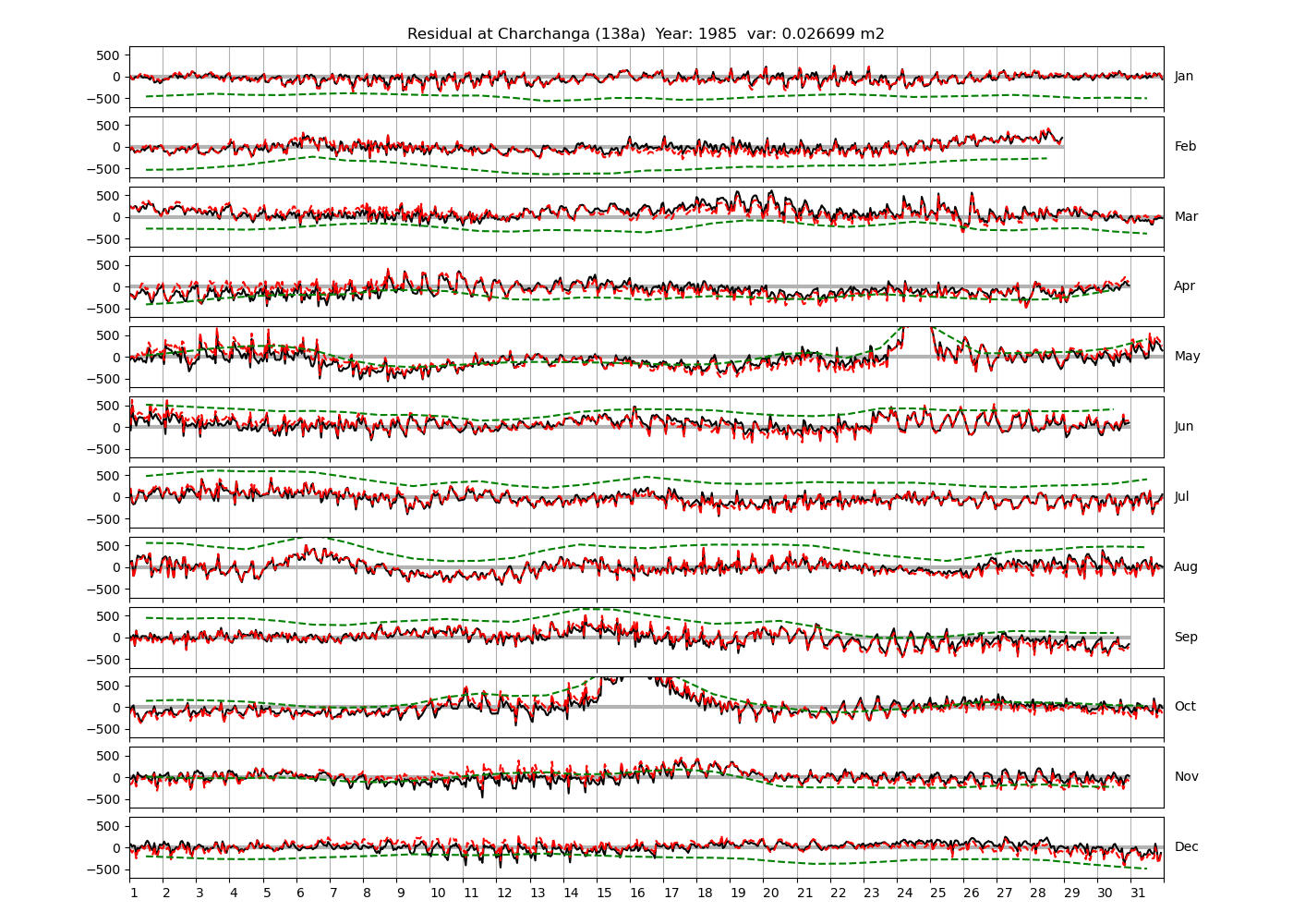
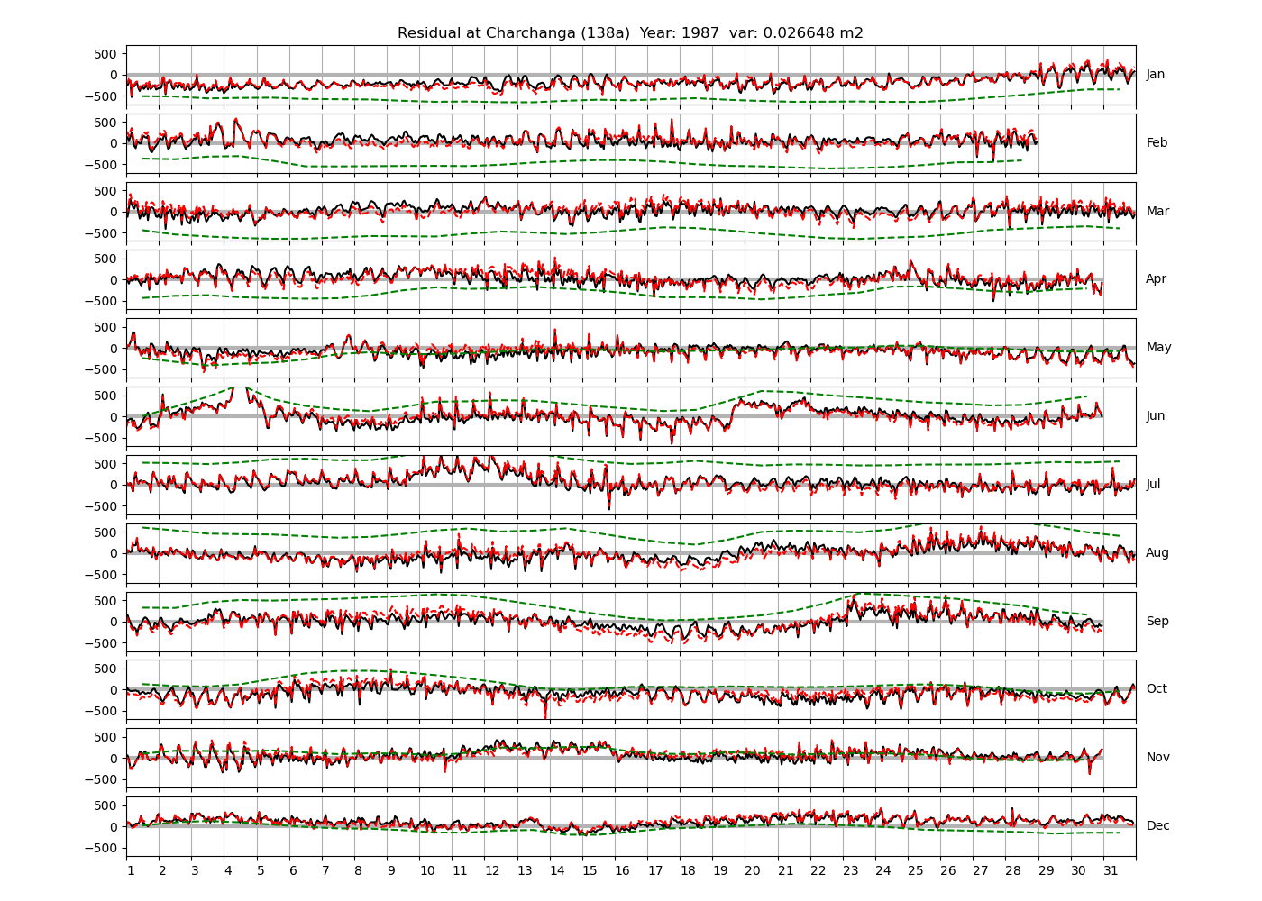
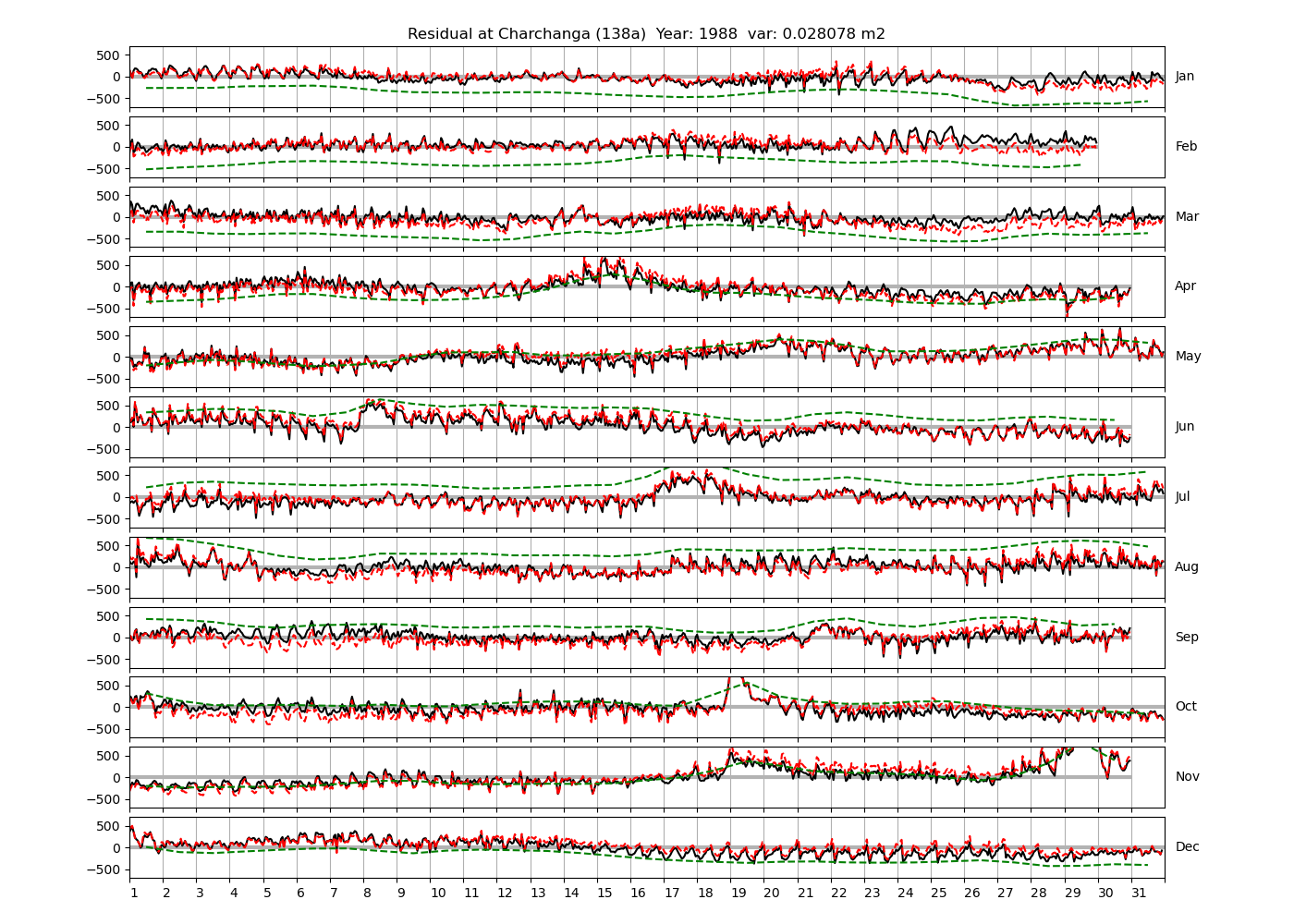
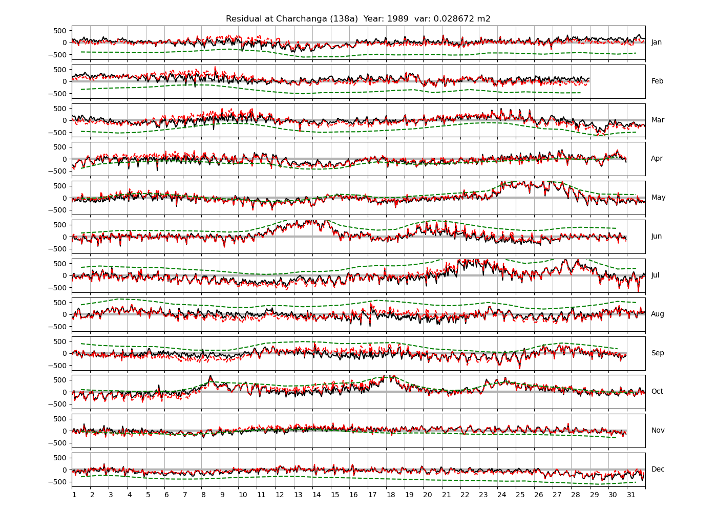
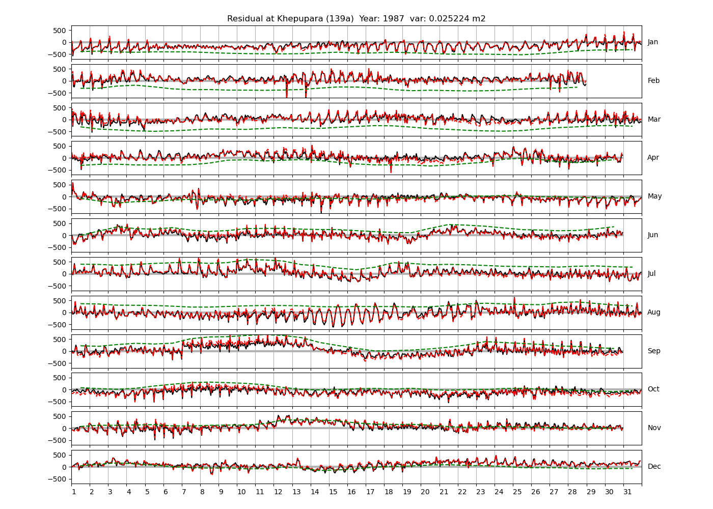
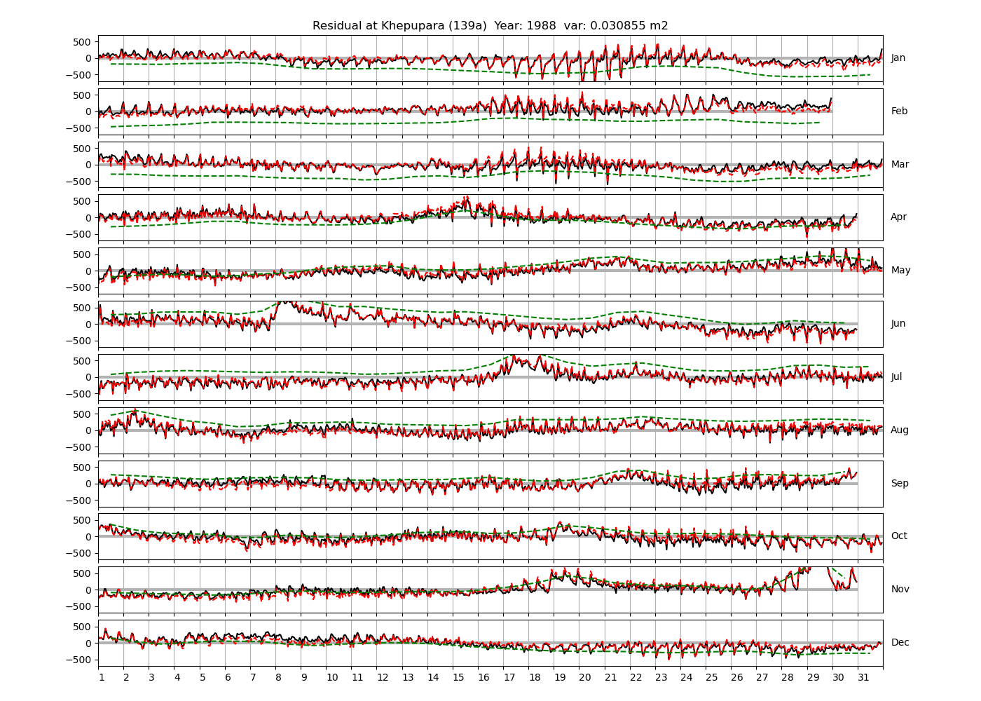
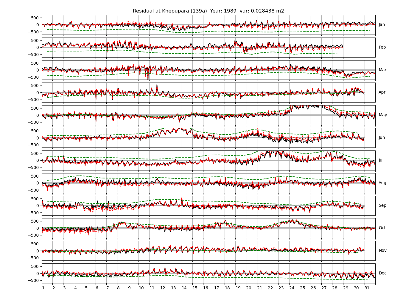
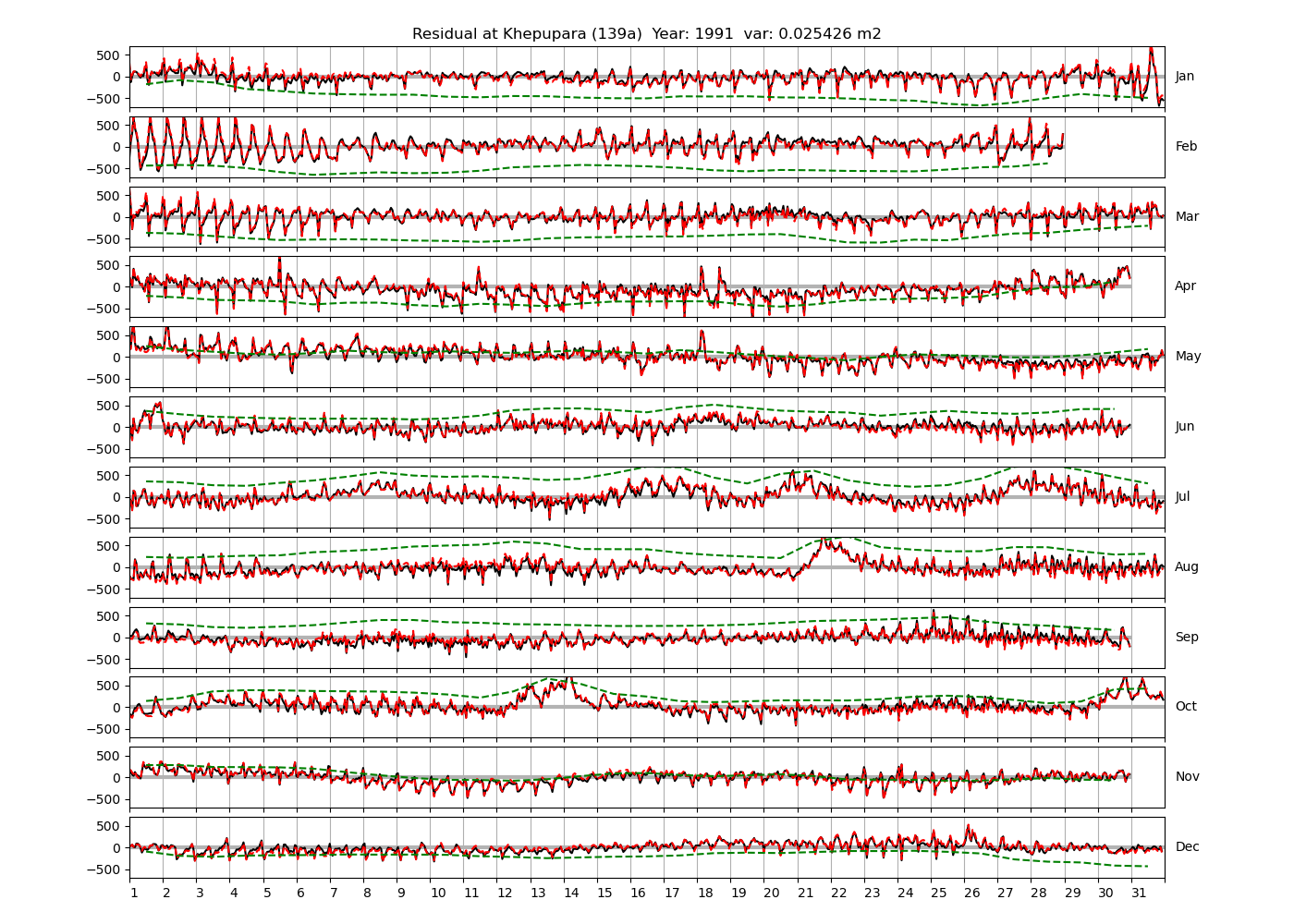
Amplitudes, monthly mean sea levels and residuals are shown for all stations. This section contains the corresponding plots for the Chittagong station with detailed captions. The figures for the remaining stations are shown in the appendix and can be accessed via the following list. Furthermore, this section also shows some more detailed plots specific to the Chittagong station.
4.1 Listing of figures
Amplitudes of tidal constituents:
- Chittagong 124a
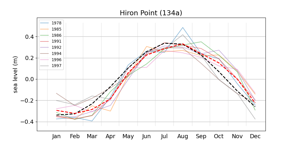
- Hiron Point 134a
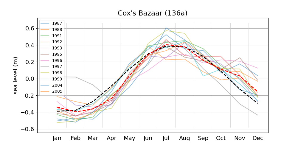
- Cox's Bazaar 136a
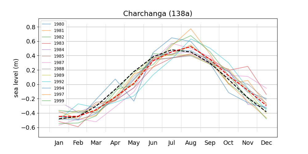
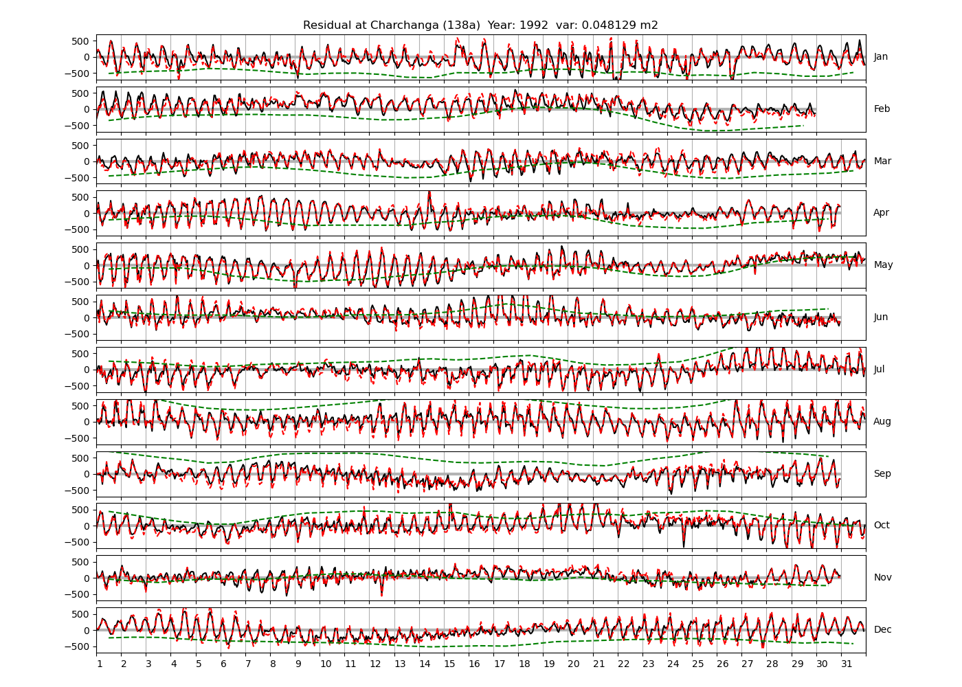
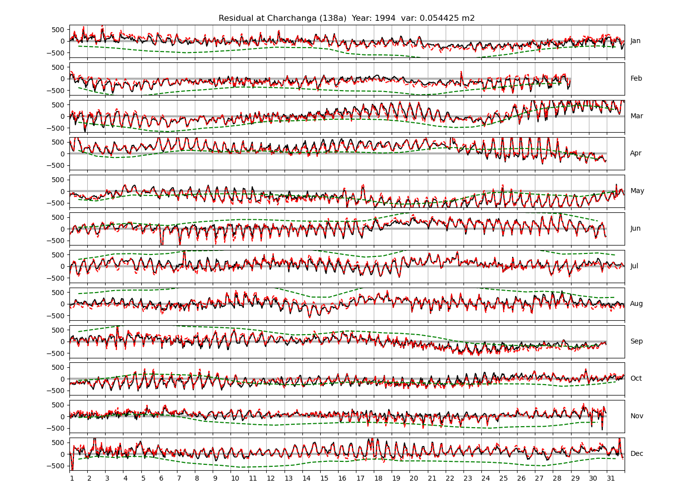
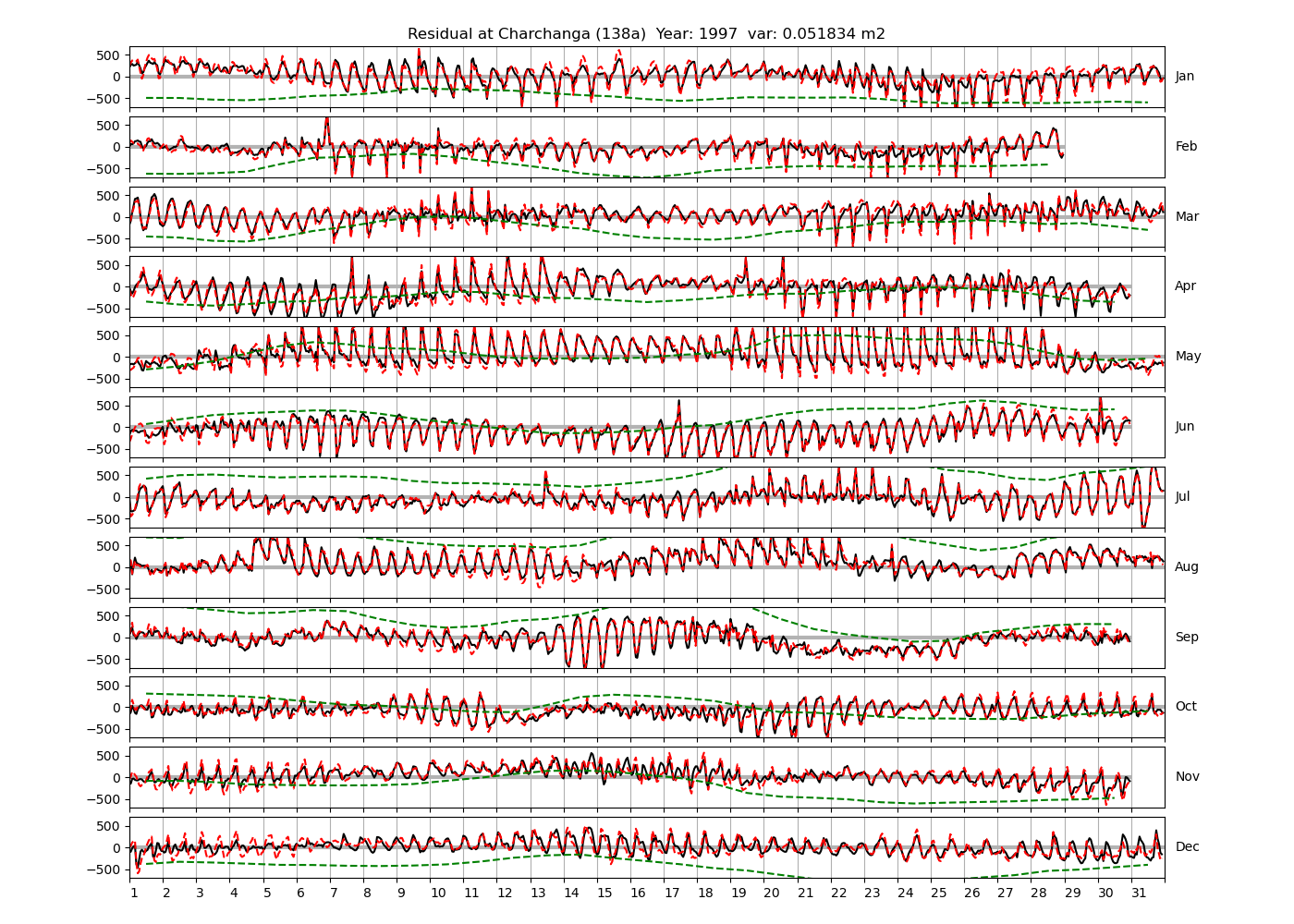
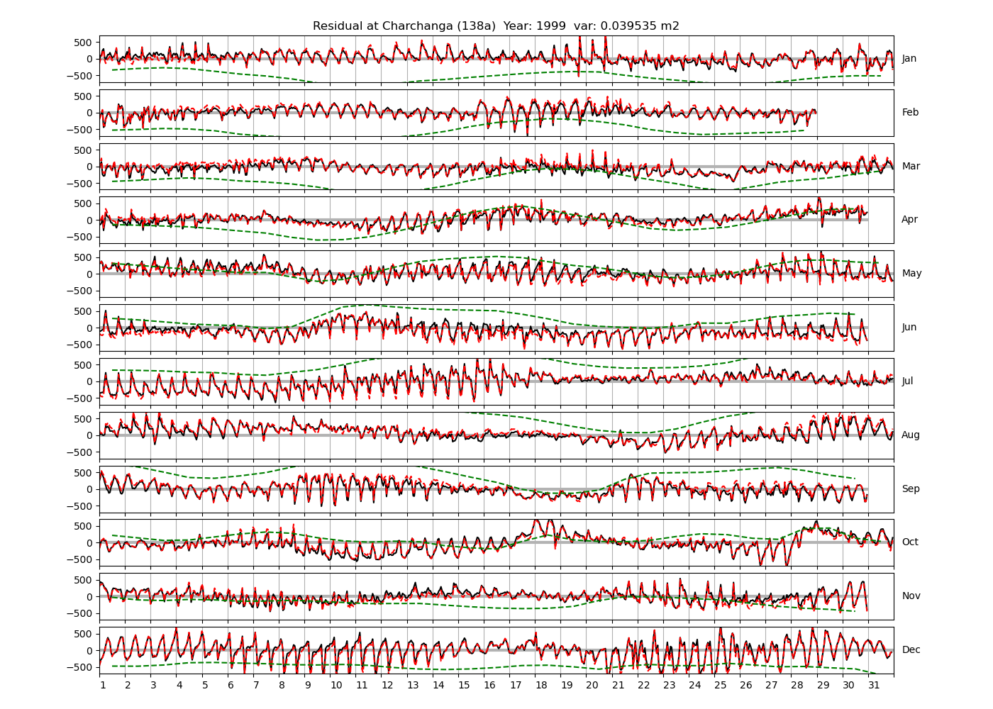
- Charchanga 138a
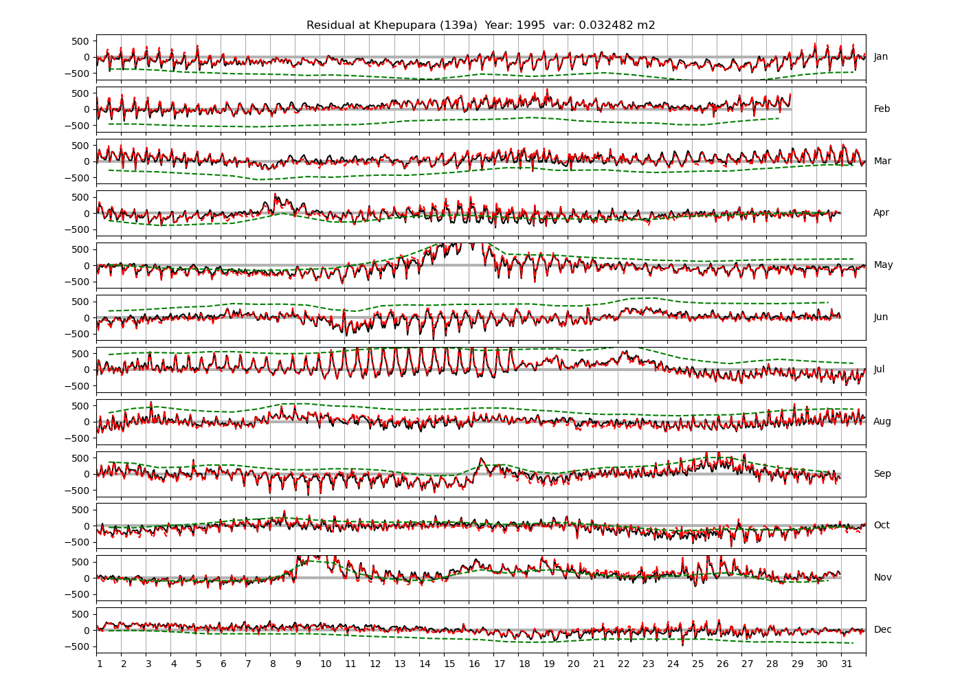
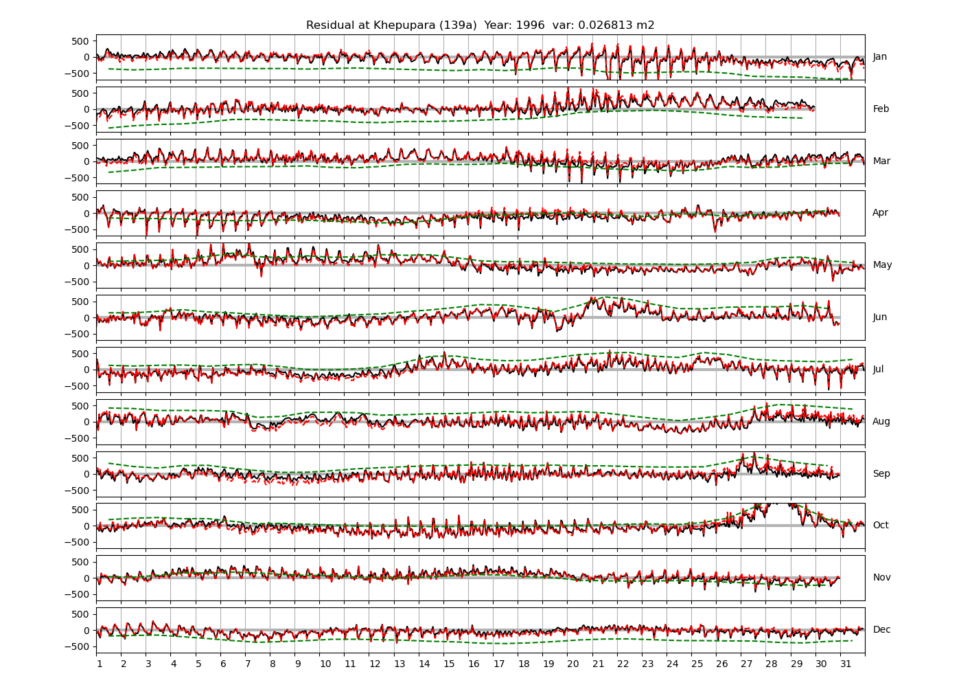
- Khepupara 139a
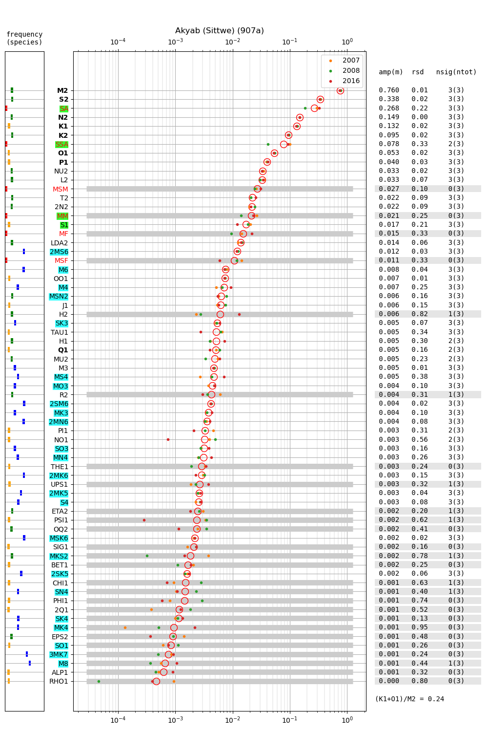
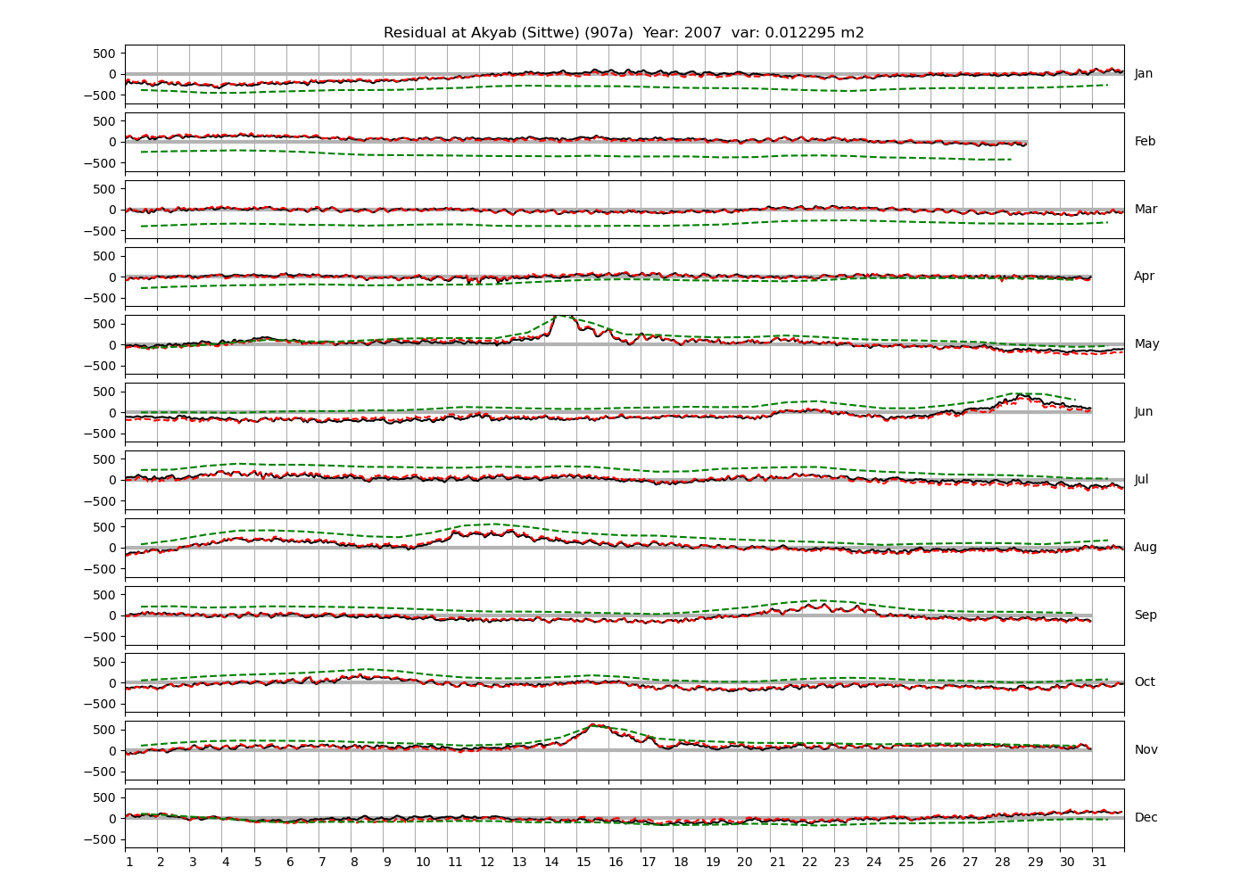
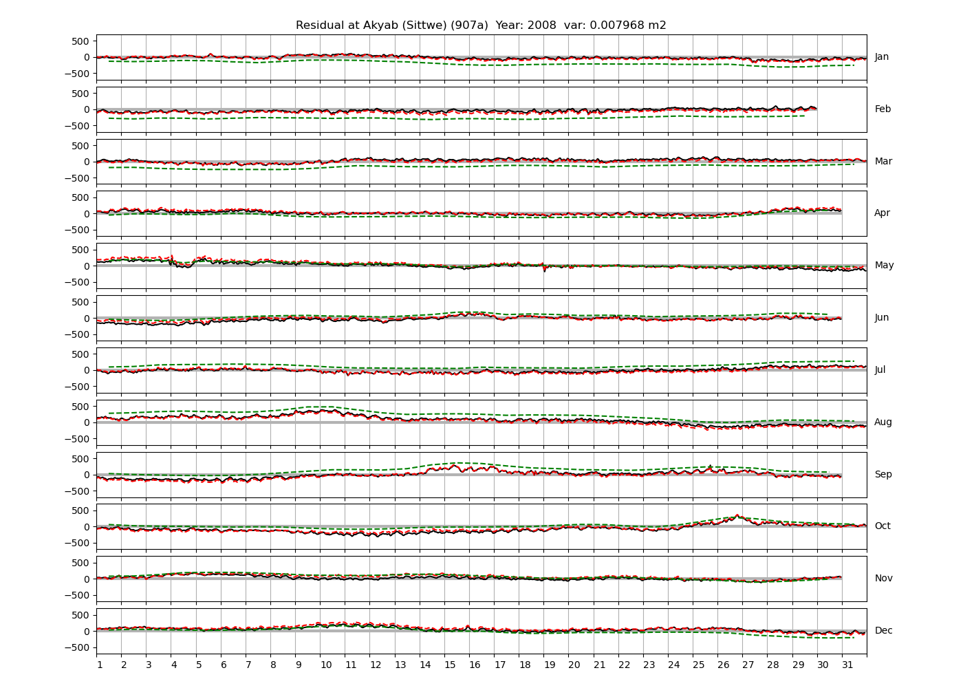
- Akyab (Sittwe) 907a
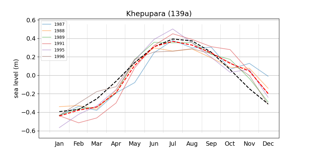
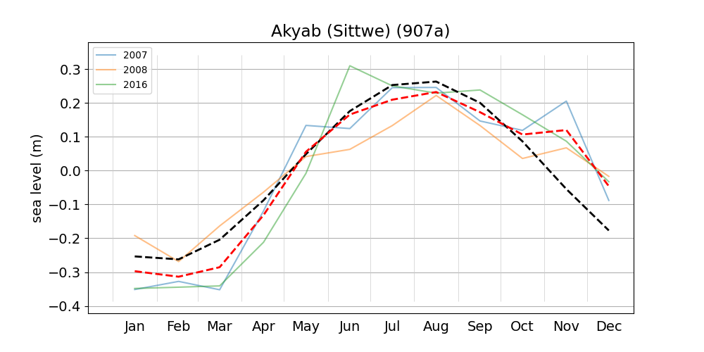
Monthly mean sea level and predictions by the solar annual constituent:
- Chittagong 124a
- Hiron Point 134a
- Cox's Bazaar 136a
- Charchanga 138a
- Khepupara 139a
- Akyab (Sittwe) 907a
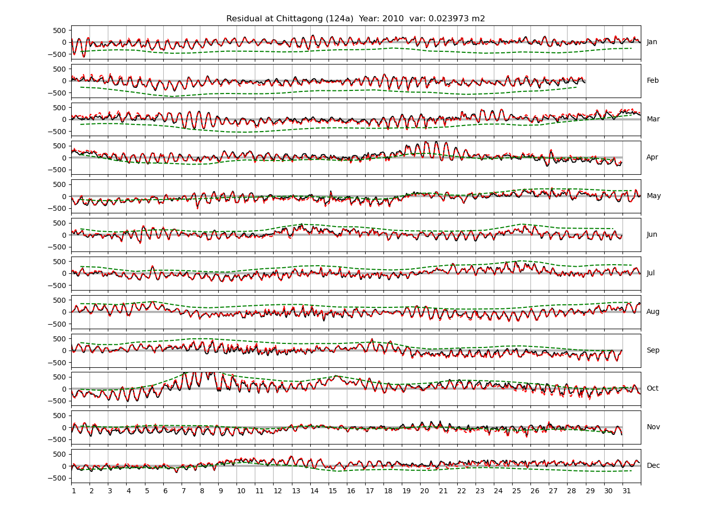
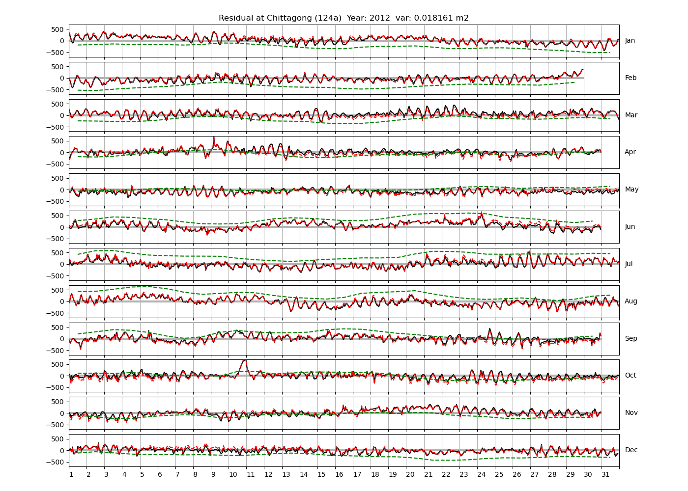
Residuals of harmonic analysis:
| Station name | Station id | Year (figure no.) |
|---|---|---|
| Chittagong | 124a | 2008 (4), 2010 (21), 2012 (22), |
| 2016 (23), 2017 (24) | ||
| Hiron Point | 134a | 1978 (25), 1985 (26), 1986 (27), |
| 1991 (28), 1992 (29), 1994 (30), | ||
| 1996 (31), 1997 (32), 1998 (33) | ||
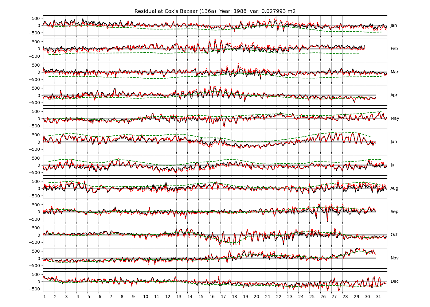
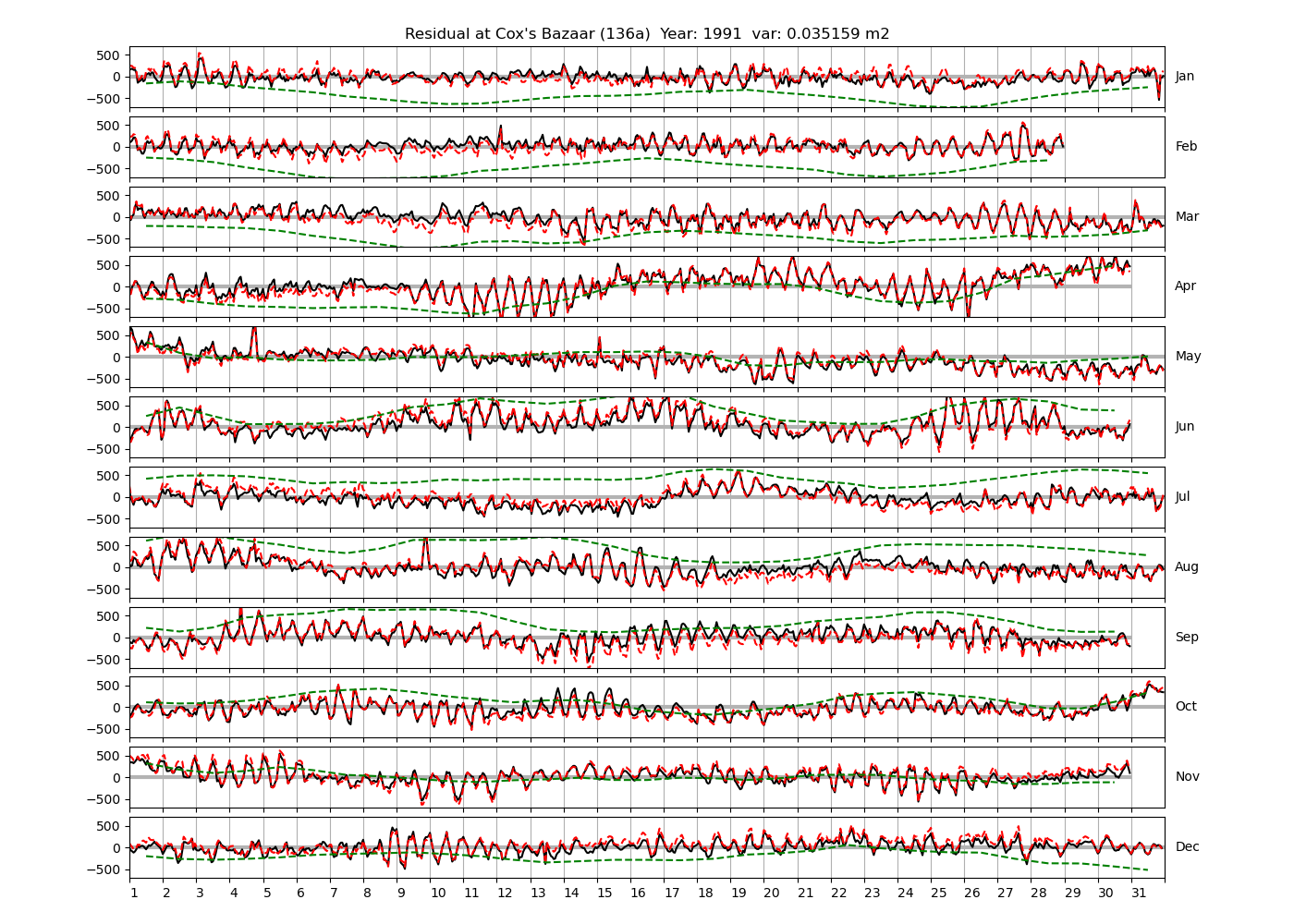
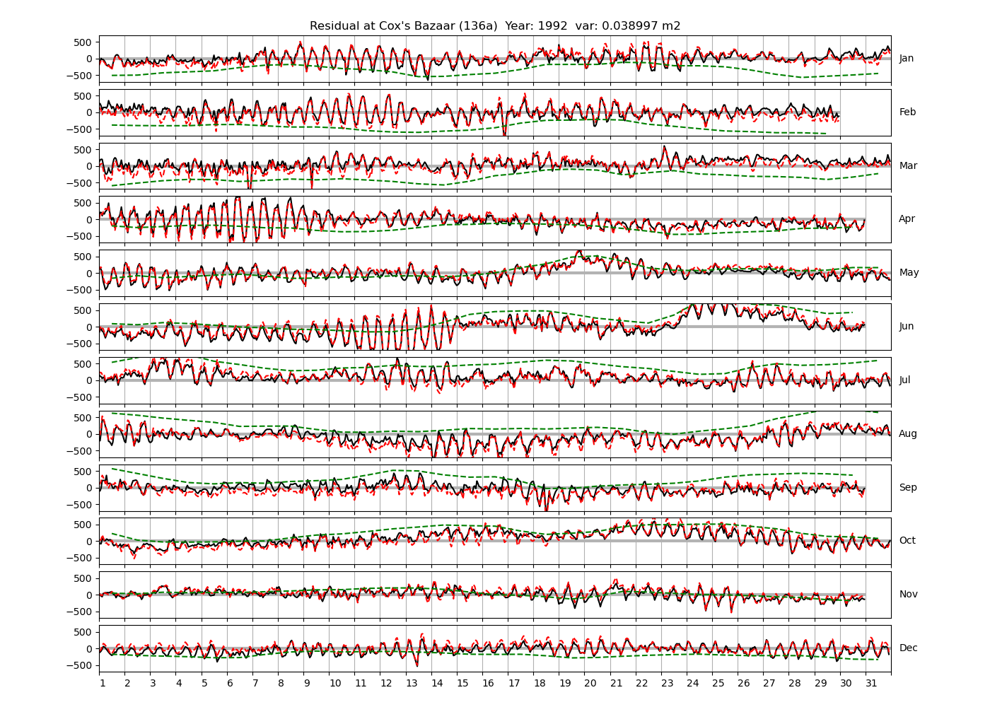
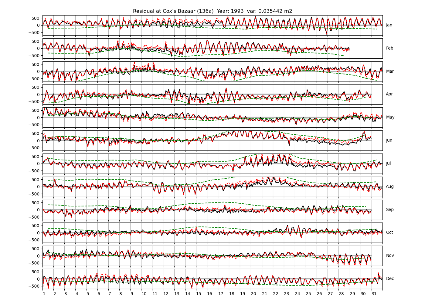
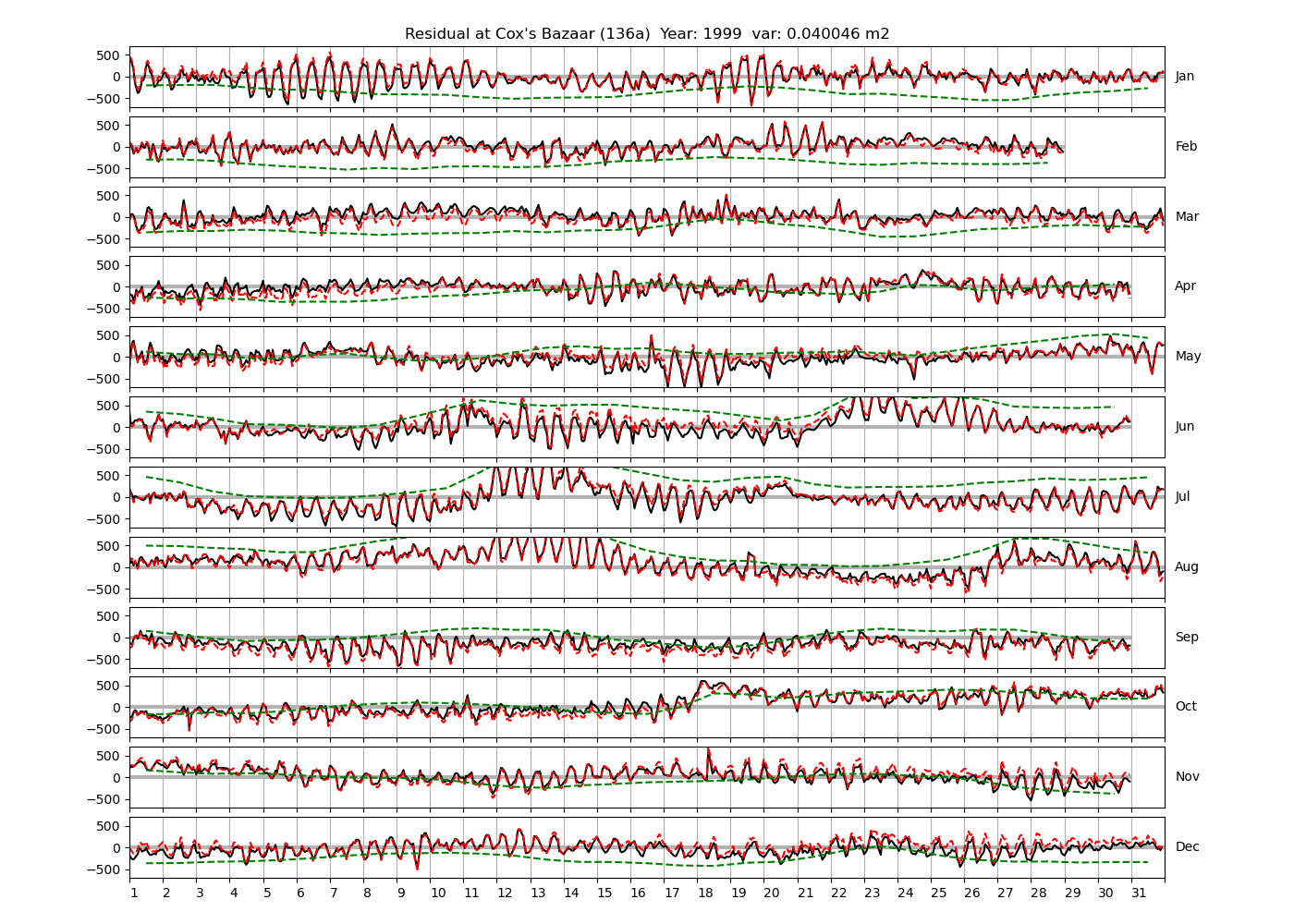
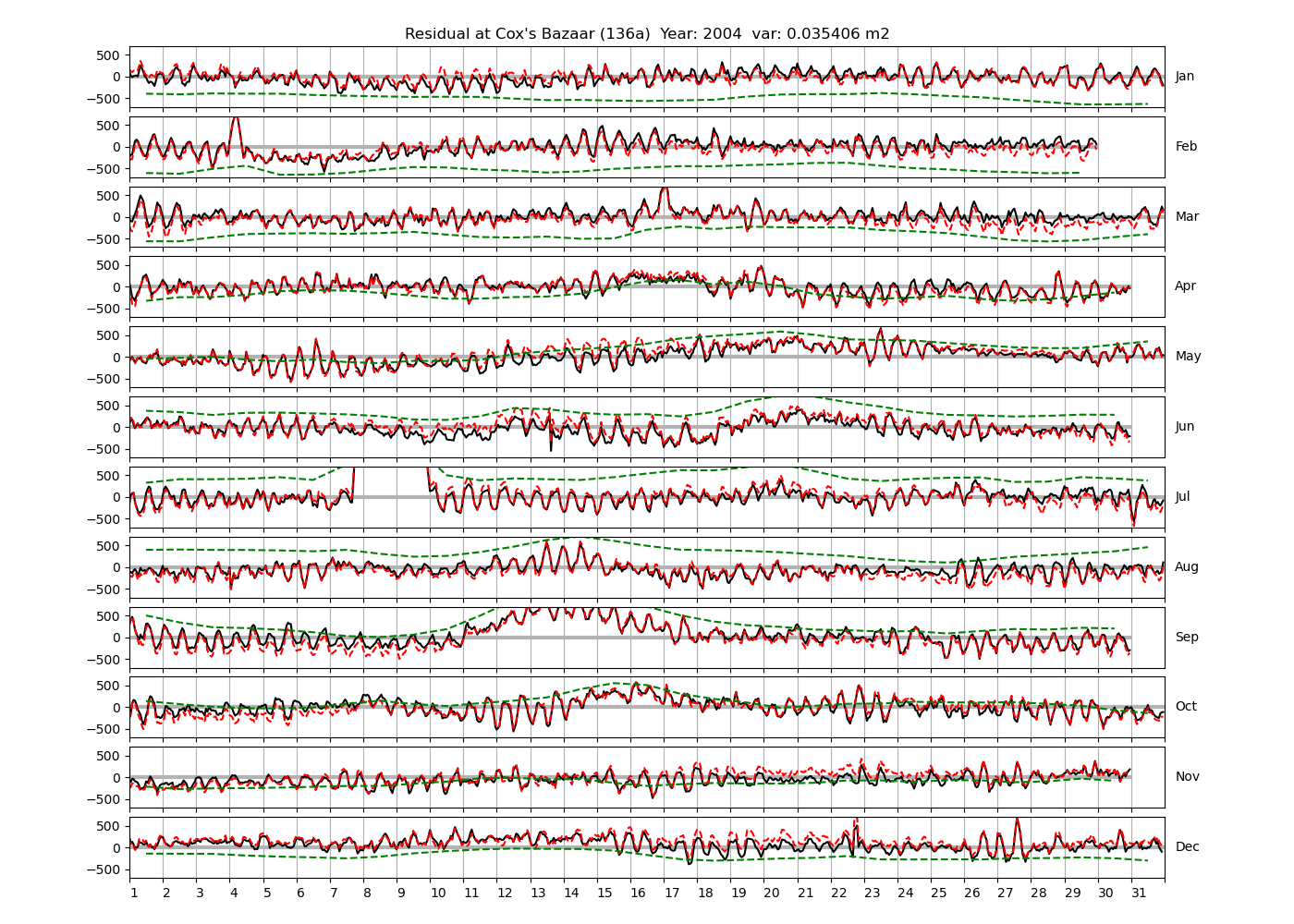
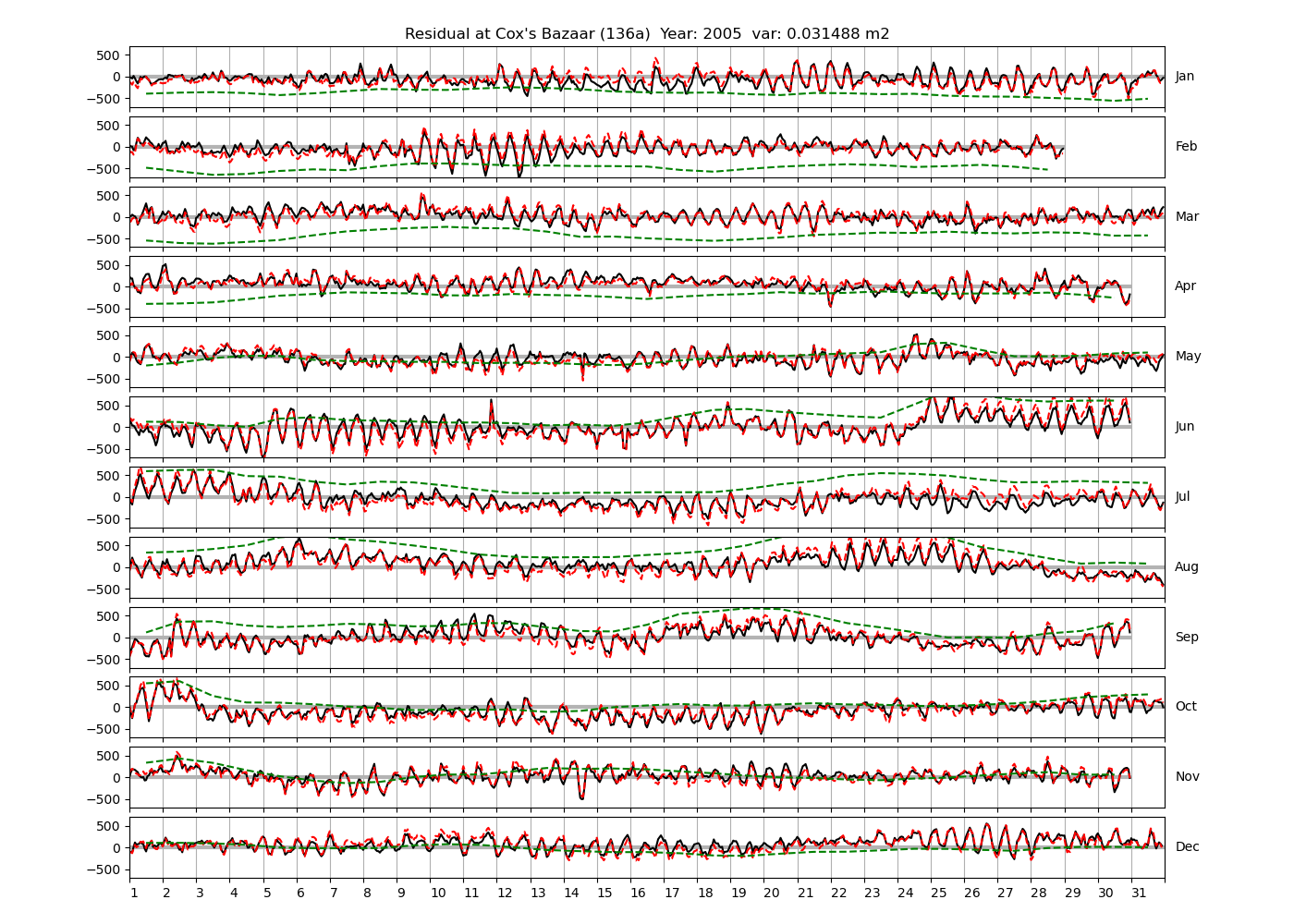
| Cox's Bazaar | 136a | 1987 (34), 1988 (35), 1991 (36), |
| 1992 (37), 1993 (38), 1995 (39), | ||
| 1996 (40), 1997 (41), 1998 (42), | ||
| 1999 (43), 2004 (44), 2005 (45) | ||
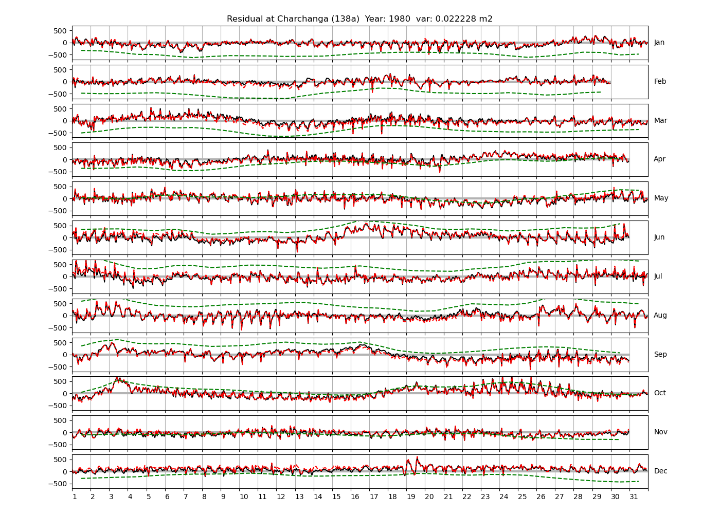
| Charchanga | 138a | 1980 (46), 1981 (47), 1982 (48), |
| 1983 (49), 1984 (50), 1985 (51), | ||
| 1987 (52), 1988 (53), 1989 (54), | ||
| 1992 (55), 1994 (56), 1997 (57), | ||
| 1999 (58) | ||
| Khepupara | 139a | 1987 (59), 1988 (60), 1989 (61), |
| 1991 (62), 1995 (63), 1996 (64) | ||
| Akyab (Sittwe) | 907a | 2007 (65), 2008 (66), 2016 (67) |
4.2 Amplitudes
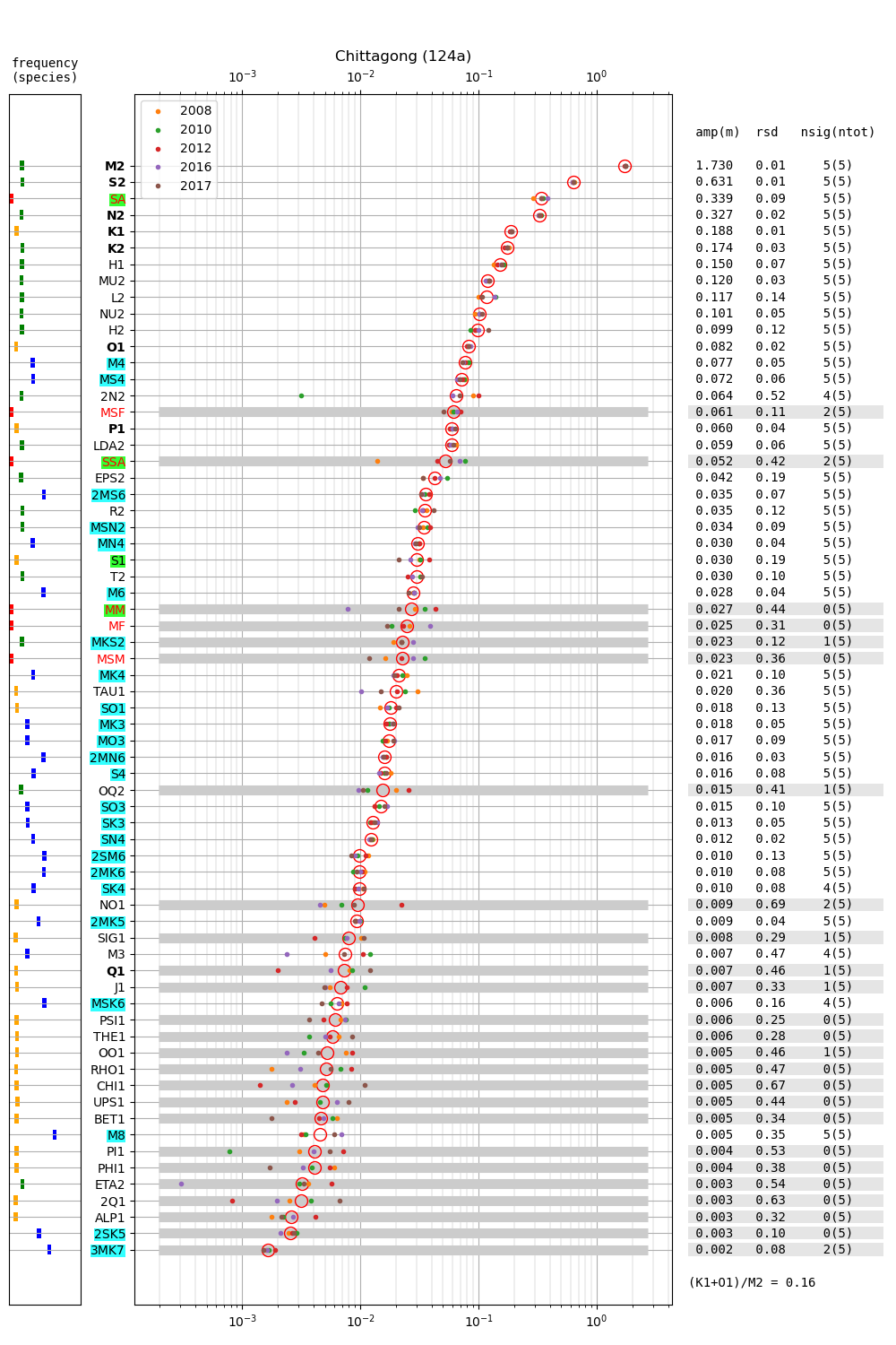
Figure 2 shows amplitudes of tidal constituents for multiple years at Chittagong (124a). The (K1+O1)/M2 mean amplitude ratio is 0.16 and the tide is generally of semidiurnal type (c.f. Parker, 2007, their page 43). At all other stations this quantity does not exceed 0.25. M2 at Chittagong (1.73m) is much larger than at the other stations. M2 ranges from 0.76m (Akyab) to 0.976 (Charchanga) at all other stations. Regarding the seasonal cycle of sea level in the region, note the relatively large amplitude of SA, whose multi-year average is more than 0.3 m. At the other stations the multi-year average of SA is 0.345 m (Hiron Point), 0.398 m (Cox's Bazaar), 0.485 m (Charchanga), 0.398 m (Khepupara) and 0.268 m (Akyab). In 4 out of 6 stations (i.e. Hiron Point, Cox's Bazaar, Charchanga and Khepupara), the mean SA exceeds the mean S2, and thus SA has the second largest mean amplitude of all constituents. Contrary to M2 and other constituents, SA is not much larger at Chittagong. This may be expected for any long-period constituent, which vary in general on larger spatial scales. The constituents H1 and H2 are 0.150 and 0.099, respectively. In Section 5 we discuss the relation of H1 and H2 to the constituents \(MA_2\) and \(Ma_2\) introduced by Corkan (1934) to represent annual modulations of M2 due to meteorological phenomena (see also Müller et al., 2014).
 for an example.
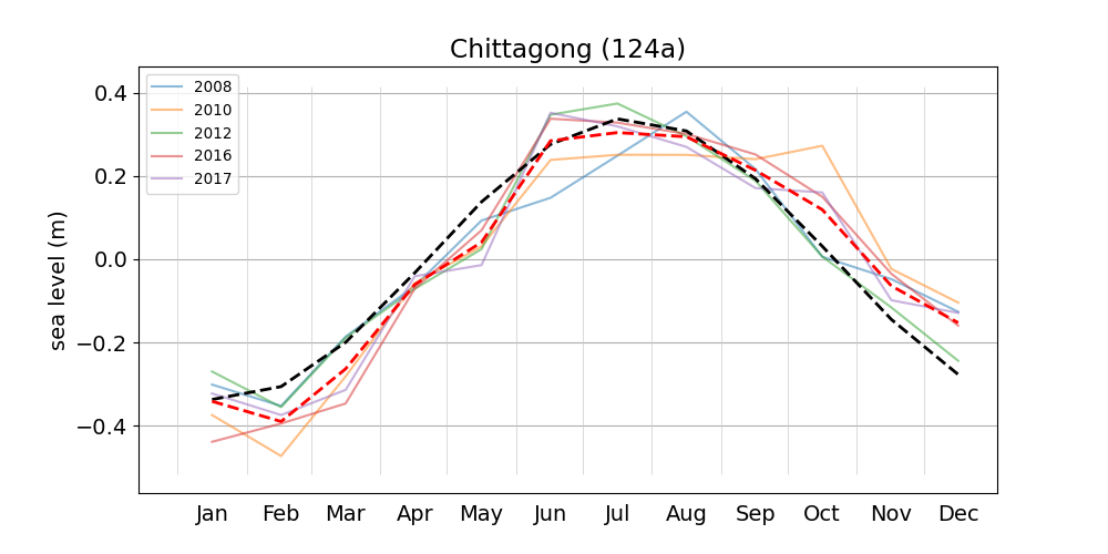
Figure 3 shows monthly mean sea level anomalies for various years at the Chittagong station. Plots for the remaining stations can be accessed from the list. The multi-year average has a range of about 0.7 m, and is reasonably well approximated by the sinusoidal contribution of the solar annual constituent SA, with an amplitude of 0.339 m (c.f. Figure 2) and an argument computed from the multi-year average Greenwich epoch and an arbitrary equilibrium argument (here for January 1, 2008). Figure 18 shows the monthly means for the station at Charchanga, where the average seasonal range is more than 0.8 m (c.f. Fig. 2 of Tazkia et al., 2017).
4.3 Residuals
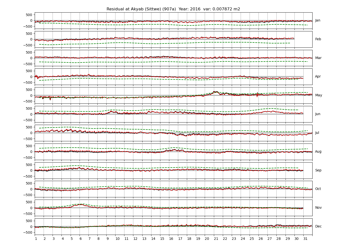
Figure 4 shows \(\zeta_{res}\) at the Chittagong (124a) station for the year 2008. All other stations and years can be accessed via the list above. As noted in Section 3 , we choose to show two different residuals throughout this blog post, one calculated with IOS Tidal Package and T_Tide. This is to highlight any possible differences arising from (1) the exclusion of non-significant constituents (as done by T_Tide in its default configuration), and (2) the different application of nodal correction numbers for predictions, as described in the companion blog post. The black line in Figure 4 shows residual heights at Chittagong for 2008, calculated with the IOS Tidal Package. The dashed red line shows T_Tide residuals omitting non-significant constituents. The dashed green line shows filtered daily sea level values obtained directly from UHSLC.
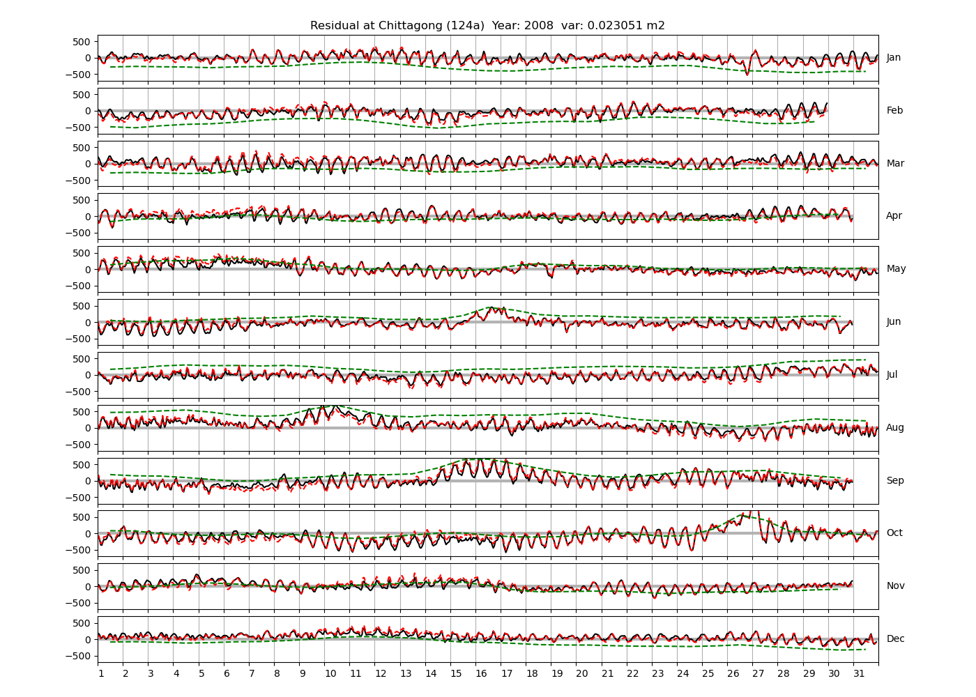
 software distributed with SLP64
  . The dashed red line shows the residual calculated with the default configuration of the T_Tide
  package, i.e. only harmonic constants above a signal-to-noise ratio larger than 2 are used for the predicted sea level. The figure is similar to the plots produced by the SLP64
  package distributed by UHSLC. Here, the monthly means are not subtracted from the monthly residuals. The length of the calendar months is indicated by a gray bar at height zero. The dashed green line shows filtered (de-tided) daily sea level values obtained from UHSLC. The annual mean was subtracted.
Apart from transient fluctuations on various temporal scales, the residual obviously oscillates with frequencies in the semidiurnal band. The variance of the residual is 0.023 \(m^2\). Table 1 lists the multi-year mean of the residual variance for all stations.
| Station | residual variance (\(m^2\)) |
|---|---|
| Chittagong (124a) | 0.0227 |
| Hiron Point (134a) | 0.0154 |
| Cox's Bazaar (136a) | 0.0407 |
| Charchanga (138a) | 0.0337 |
| Khepupara (139a) | 0.0282 |
| Akyab (Sittwe) (907a) | 0.0094 |
The variances of the observed, predicted and residual time series for the year 2008 at Chittagong are
- observed: 1.840 \(m^2\)
-
predicted:
- IOS Tidal Package: 1.819 \(m^2\)
- T_Tide: 1.813 \(m^2\)
-
residual:
- IOS Tidal Package: 0.023 \(m^2\)
- T_Tide: 0.027 \(m^2\)
The variances of the observed and predicted time series are shown as function of the tidal species in Figure 5. The line for \(\zeta_{pred}\) is computed with IOS Tidal Package (all constituents). The units of the horizontal axis are frequencies corresponding to the period of a mean lunar day, i.e. about 24.8412 hours (c.f. Parker, 2007, their table 2.1. on p.29). The variance shown is accumulated within each band. The observed variance has a maximum of 1.742 \(m^2\) at the semidiurnal band, and is about 0.03 \(m^2\) in the diurnal band. It is noteworthy that the variance is generally higher at even multiples of \(f_L=\omega_L/(2\pi)\). We speculate that this is because there is far more energy in the semidiurnal band than in the diurnal band (both in the water level and the residual, as shown below), and that the energy at higher frequencies is dominated by overtides of the semidiurnal species.
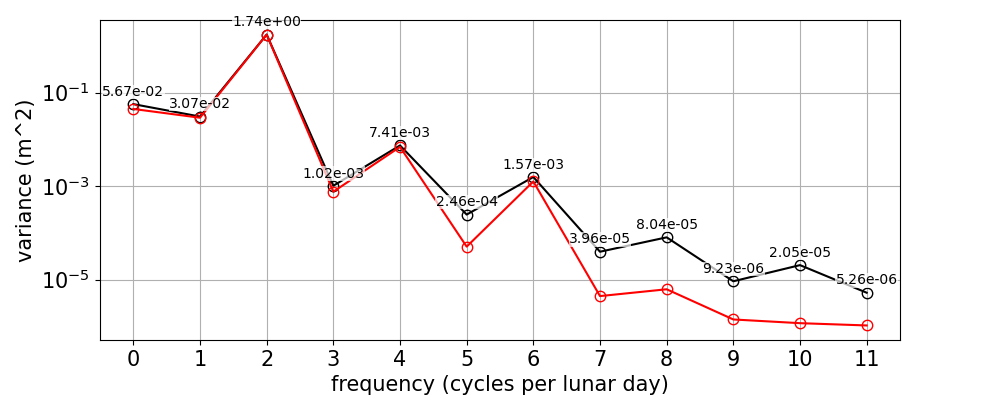
Figure 6 shows how the variance of the residual is distributed over the tidal species. The accumulated variance in the low-frequencies (up to 0.5*\(\omega_L\)) is about 0.012 \(m^2\), and about 0.008 \(m^2\) in the semidiurnal band. Like for the observed and predicted time series, the variance of the residual is generally higher for even multiples of the lunar frequency. However, the energy in the residual is highest in the low-frequency band.
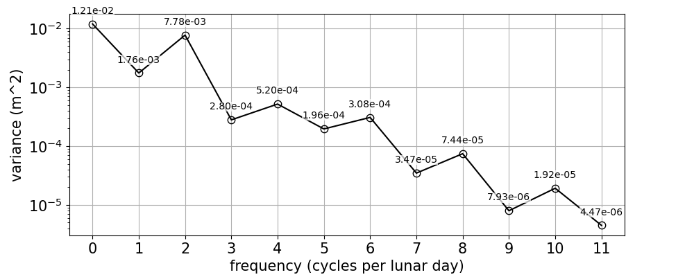
Figure 7 shows a discrete Fourier transform of the residual time-series in the low-frequency band. There is a lot of energy between the semi-annual and monthly frequencies, presumably due to meteorological phenomena. Note that the resolution in frequency space is about 1/y. Higher resolution of the discretization would require time series of larger intervals than one year.
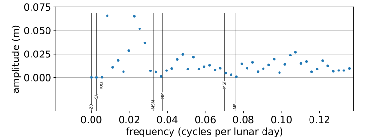
Figure 8 shows a discrete Fourier transform of the residual in the semi-diurnal band. There is some energy in frequencies which could be resolved with time-series of 366 days. For example, the shallow-water constituent ST2 is in between the resolved constituents \(\epsilon_2\) (with shallow-water equivalent \(MNS_2\), see table A.1. of Parker 2007) and the lunar constituent \(2N_2\) (shallow-water equivalent \(2NM_2\)). The frequency interval \(ST2-\epsilon_2\) and (\(2N_2-ST2\)) is larger than required by the Rayleigh criterion, as can be seen from Figure 8 by comparison to the interval between any two narrowly spaced black vertical lines indicating resolved frequency pairs. Configuring T_Tide to include 2NS2, ST2 and 2SM2 decreases the total residual variance from 0.023 \(m^2\) to 0.021 \(m^2\), and has no clear visible effect on the residual time series (not shown).
5 Summary and discussion
We use two popular harmonic analysis tools, IOS Tidal Package and T_Tide, to compute harmonic amplitudes and residuals at 6 tide gauges in the north-eastern Bay of Bengal. The data was obtained in preprocessed form from UHSLC and/or other third parties (see acknowledgements 6 ). The software packages produce slightly different results, and at this stage we do not attempt to justify the choice of one package over another. In fact, the results presented here are a first attempt to gain intuition about the usefulness of e.g. the confidence intervals computed by T_Tide.
Overall, the results agree with previous studies about tides in the region. The M2 amplitude is a local maximum at Chittagong, consistent with e.g. Sindhu and Unnikrishnan (2013). Note that Fig. 5 of Sindhu and Unnikrishnan (2013) shows a slightly higher M2 amplitude at station Sagar Roads, located along 88.05E, which approximately coincides with the left border of our map. This station was not available to us.
Most residual time series have large unresolved fluctuations, probably due to the wide continental shelf and shallow water adjacent to the GBM delta. Preliminary results with shorter time series yield a smaller residual and will be presented in future work.
Tazkia et al. (2017) used a sliding window of 2 months to compute temporally varying M2 amplitudes for the north-eastern Bay of Bengal. They found that seasonal changes typically range from 10 cm to 20 cm in amplitude, and are largest in the coastal and estuarine areas of the Bengal delta. Observations and numerical modelling suggest a close correspondence between the seasonal cycle of the M2 amplitude and the seasonal cycle of water level.
Müller et al. (2014) studied the seasonal cycle of M2 produced by a global numerical ocean model, validated against 19 years of satellite altimeter and multiyear tide-gauge records. They use two methods to describe the seasonal variation of M2. The first method uses sliding windows, which is the method later adapted by Tazkia et al. (2017) to study the region around the GBM delta. The second method builds on the concepts of classical harmonic analysis and interprets the seasonal modulation of M2 as induced by a fictitious celestial body (or satellite). This has the conceptual advantage that M2 can be expressed by true harmonic constants, which are by definition independent of time, but requires the introduction of additional constituents to express the temporal modulation. The practice of defining a "meteorological constituent" which modulates M2 at an annual frequency, goes back at least to Corkan (1934) (see Müller et al., 2014, for reference). Müller et al. (2014) show two examples for which the use of constituents \(\alpha_2\) and \(\beta_2\) (named H1 and H2 in the IOS Tidal Package ) yield unsatisfactory results, i.e. in the case where the annual cycle of the amplitude is not approximately sinusoidal.
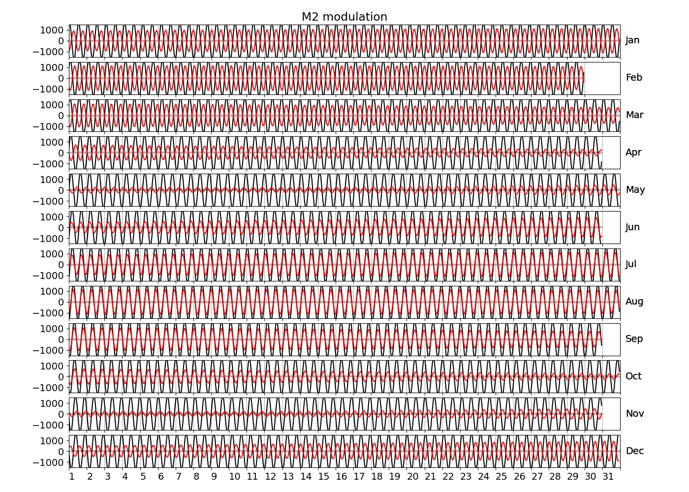
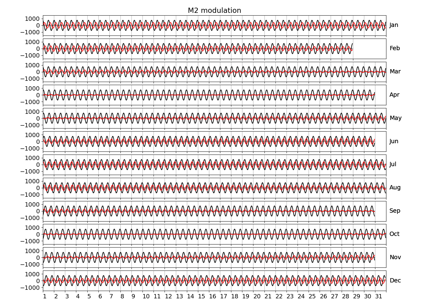
Tazkia et al. (2017) find observed absolute seasonal differences between M2 amplitudes of 8 cm at Hiron Point and 21cm at Charchanga. We find amplitudes of 4.4 cm and 4.5 cm for constituents H1 and H2, respectively, at Hiron Point, yielding a maximum value of 8.9 cm amplitude at times of constructive interference between H1 and H2. We find amplitudes of 9.2 cm and 2.9 cm for constituents H1 and H2, respectively, at Charchanga, yielding a maximum value of 12.1 cm amplitude for combined H1 and H2. It is essential to note, however, that the maximum amplitude of H1+H2 does not necessarily induce an amplitude increment of the same magnitude on top of M2. In fact, whether this is the case depends on the phase lag between M2 on the one hand, and H1+H2 on the other hand. To see this, compare Figure 9 and Figure 10, which show exemplary years at Chittagong and Hiron Point. In Figure 9, the red line shows the sum of contributions from H1+H2, multiplied by a convenient factor of 5 for better visibility. For the shown station and year, H1 and H2 have amplitudes of 0.15 m and 0.099 m, respectively. They interfere constructively with each other in February and August. The composite H1+H2 interferes with M2 destructively in winter and constructively in summer. Note that the composite H1+H2 is approximately in phase or antiphase with M2 at times where the amplitude of H1+H2 is large. In other words, the amplitudes of H1 and H2 can be added to the amplitude of M2 to obtain the total amplitude of modulation. To see that this is generally not the case, consider Figure 10, which shows the modulation at Hiron Point in 1985. When the amplitude of H1+H2 is large (times of constructive interference), H1+H2 is approximately in quadrature with M2, i.e. shifted in phase by approximately \(\pi/2\) with respect to M2. Hence the amplitudes of H1 and H2 cannot simply be added to M2 to obtain the total amplitude modulation. In fact, the total amplitude modulation is significantly lower (not shown).
A more systematic quantification of the induced total modulation, and hopefully some error correction, is deferred to future work, which will be presented along with harmonic analysis using monthly (or 2-monthly) sliding windows.
5.1 Further questions
In the context of the second method used by Müller et al. (2014), i.e. the method involving H1 and H2, two questions arose during the writing of this blog post. The first relates to the exact definition of H1 and H2, the second arises from what appears to be a mistake in Eq. (22) of Müller et al. (2014). The first issue is discussed in the remainder of this section. The second issue is discussed in Appendix B.
5.2 Inconsistent definition of tidal constituents
We noted an apparent inconsistency in the naming conventions of tidal constituents. The solar annual constituent named SA seems to be defined alternately as the inverse of a tropical year and an anomalistic year. For example, in table A.1 of
Parker (2007), SA has Cartwright numbers (0,0,1,0,0,0) and hence the period of a tropical year (see also our table 2). In general, governmental agencies in the U.S. seem to use the tropical year for SA. As an example, see the listing of tidal constituents 
Their table 1 contains a note stating that (quote:) "symbols refer to the rate of change in mean longitude", and further above in their table 1, the symbol \(h\) is associated with the sun. It seems that the usage of \(h\) in both Schureman (1958) and Corkan (1934) is consistent, and hence that Corkan (1934) did not suggest the involvement of the solar perigee. This is inconsistent with the naming convention of Müller et al. (2014), who state that the annual constituents proposed by Corkan (1934) are sometimes referred to as \(\alpha_2\) and \(\beta_2\) in the literature. We were unable to obtain their reference ( Hartmann and Wenzel 1995) free of charge, but e.g. Parker (2007) includes at least \(\alpha_2\) in their tables A.1 and A.2, with Cartwright numbers (2,0,-1,0,0,1), i.e. in terms of frequency
where (from Parker, 2007, their table 2.1)
| Symbol | Description |
|---|---|
| \(1/f_L\) | Mean lunar day |
| \(1/f_2\) | Period of solar declination (tropical year) |
| \(1/f_5\) | Period of perihelion (~20,940 years) |
The inclusion of \(f_5\) seems to deviate from what
Corkan (1934) proposed. Searching for further clarification, we found a tidal constituent list 
Despite their appearance neither [MA2 nor MB2], nor constituents of other species which include A and B, are compound constituents – there are no constituents A or B to form a compound. They are constituents whose speeds differ by one cycle a year from that of M2. The A in MA2 was intended to signify the Annual differences. MB2 was originally called Ma2 but this became ambiguous when spoken, or typed on computers without lower case, and so it was initially changed to MA2*. However, this in turn was thought to be clumsy and hence MB2 was finally adopted. Although theoretically they should have the same values of u and f as M2, they are so small that they are commonly treated as having values of u = 0 and f = 1.
Only after reading this paragraph, the author noted that the constituent Sa in the IHO list 
Do the differences between MA2 and MB2 on the one hand, and \(\alpha_2\) and \(\beta_2\) (or its shallow water equivalent) on the other hand, matter in practical applications with time series of 366 days? Given the interval which would be necessary to separate the pairs, i.e. the period of the rotation of the perihelion around the sun (~20940 years), this may not be the case.
6 Acknowledgements
We thank UHSLC, the director of Meteorology CIVAIR at the SEEB International Airport of the Sultanate of Oman, and the Bangladesh Inland Water Transport Authority (BIWTA) for providing data. We thank the authors of IOS Tidal Package and T_Tide for providing their software. Figures in this blog post have been prepared with matplotlib 


7 Appendix A
8 Appendix B
Müller et al. (2014) present an equation for the modulation of M2 in their Eq. (22). After some initial attempts to reproduce their result, we suspect that their expression may contain an error. Corrections and comments via E-mail are appreciated. We start at their expression for \(\zeta(t)\) in Eq. (21) and attempt to reorder terms to a form that is as similar as possible to their expression in Eq. (22). To simplify manipulation, let
Then Eq. (21) of Müller et al. (2014) can be written as
In summary,
where
Setting \(\epsilon(t)=0\) yields
Setting our auxiliary variables back to the ones used by Müller et al. (2014) yields for \(\delta(t)\)
which is identical to Eq. (22) of Müller et al. (2014). However, the term \(\epsilon(t)\) is generally non-zero, which is unaccounted for in the presentation of Müller et al. (2014).
References
- Caldwell, P.C., Merrifield, M.A., Thompson, P.R., 2015: Sea level measured by tide gauges from global oceans — the Joint Archive for Sea Level holdings (NCEI Accession 0019568), Version 5.5, NOAA National Centers for Environmental Information, Dataset, doi:10.7289/V5V40S7W.
- Caldwell, P.C., 2015: Hourly Sea Level Data Processing and Quality Control Software: Version for Linux Operating Systems. SLP64 User Manual
- Cartwright, D.E., Edden, A.C., 1973: Corrected tables of tidal harmonics.
- Corkan, R.H., 1934: An annual perturbation in the range of tide.
- Dube, S.K., Rao, A.D., Sinha, P.C., Murty, T.S., 1997: Storm surge in the Bay of Bengal and Arabian Sea the problem and its prediction.
- Eaton J.W., Bateman D., Hauberg S., Wehbring R., 2020: GNU Octave version 6.1.0 manual: a high-level interactive language for numerical computations.
- Foreman M.G.G, 1977: Manual for Tidal Heights Analysis and Prediction. Pacific Marine Science Report 77-10, Institute of Ocean Sciences, Patricia Bay, Sidney, B.C., 58 pp. (2004 revision)
- Foreman M.G.G, Henry R.F, 1989: The harmonic analysis of tidal model time series
- GEBCO Compilation Group, 2020: GEBCO 2020 Grid (doi:10.5285/a29c5465-b138-234d-e053-6c86abc040b9).
- Godin, G., Taylor, J., 1973: A simple method for the prediction of the time and height of high and low water.
- Godin, G., 1972: The Analysis of Tides.
- Han, W., Webster, P.J., 2002: Forcing mechanisms of sea level interannual variability in the Bay of Bengal.
- Harris, C.R., Millman, K.J., van der Walt, S.J., others, 2020: Array programming with NumPy.
- Hartmann, T., Wenzel, H.G., 1995: The HW95 tidal potential catalogue.
- Hunter, J.D., 2007: Matplotlib: A 2D Graphics Environment.
- Intergovernmental Oceanographic Commission, 1992: Joint IAPSO-IOC Workshop on Sea level measurements and quality control, Paris, 12-13 October 1992. (ed. N.E.Spencer)
- Müller, M., Cherniawsky, J.Y., Foreman, M.G., von Storch J.S., 2014: Seasonal variation of the M2 tide.
- Parker, B.B., 2007: Tidal analysis and prediction. NOAA Special Publication NOS CO-OPS 3, U.S. Department of Commerce, 378 pp.
- Pawlowicz, R., Beardsley, B., Lentz, S., 2002: Classical tidal harmonic analysis including error estimates in MATLAB using T_TIDE.
- Schureman, P., 1958: Manual of harmonic analysis and prediction of tides.
- Sindhu, B., Unnikrishnan, A.S., 2013: Characteristics of tides in the Bay of Bengal.
- Tazkia, A.R., Krien, Y., Durand, F., Testut, L., Islam, A.S., Papa, F., Bertin, X., 2017: Seasonal modulation of M2 tide in the Northern Bay of Bengal.
