Storm surge simulations using ROMS in 2-d mode with grid nesting and wetting/drying

Numerical storm surge modeling for risk assessment has, in the past, been mainly conducted with 2-dimensional, i.e. depth-integrated ocean models. Two examples are ADCIRC (e.g. Westerink et al. 2008; Taflanidis et al. 2013) and SLOSH (e.g. Lin et al. 2010; Forbes et al. 2014). These models allow stochastic storm surge risk assessment, for which hundreds or thousands of model runs are evaluated to produce large sets of inundation events. Three-dimensional frameworks for storm surge modeling exist ( Xu et al. 2016; Mooney et al. 2016; Mooney et al. 2019; Olabarrieta et al. 2012; Marsooli et al. 2017; Warner et al. 2017), and these are e.g. used to study ocean-atmosphere interaction and sediment transport for individual storms. In this post we describe our experiences configuring the Regional Ocean Modeling System (ROMS, Shchepetkin and McWilliams, 2005), a comprehensive three dimensional model, as a two-dimensional model capable of producing relatively efficient preliminary estimates of inundation depths caused by storm surges. The long-term motivation is to establish a modeling framework that requires minimal adjustment for switching between stochastic 2-d modeling on the one hand, and comprehensive 3-d case studies on the other hand. As computing power increases, the former will gradually adopt the complexity of the latter, and the use of a common code base seems attractive.

ROMS is a free-surface, terrain-following, primitive equations ocean model. The model is widely used in regional and coastal oceanography. At least 4 versions of ROMS are maintained by groups of scientists based in various institutions (DMCS at Rutgers , IGPP at UCLA , LEGOS , USGS ). To our knowledge, the majority of studies investigating the ocean's response to severe storms, some of which also study ocean-atmosphere interaction, has been produced using the version maintained by USGS. That version is a component of the Coupled-Ocean-Atmosphere-Wave-Sediment Transport (COAWST) Modeling System, and is coupled to atmospheric, wave and sediment models. Our understanding is that COAWST mainly originated from the desire to study sediment transport. We further speculate that a 2-dimensional model is of rather limited use to sedimentologists, given that the interactions between wind forcing at the surface, and transport processes in the bottom boundary layer of the ocean must be resolved by the numerical ocean model. On the other hand, the need for very high (lateral) resolution models, which often entails the necessity to use nested grids, and also the requirement to model wetting and drying of land, seems to constitute some overlap between the different lines of research.

In this blog post we describe a toy model that simulates the storm surge caused by Hurricane Sandy in New York City. We focus less on obtaining realistic results, and more on describing and testing the basic computational components of the modeling framework that are of fundamental importance for efficient two-dimensional inundation modeling:

• Two-dimensional (depth-integrated) setup
• Grid nesting
• Wetting/drying functionality
• Wind forcing
• Tidal forcing

We test our toy setup by:

• Comparison of the modelled tidal elevation at Battery Park to observations.
• Comparison of the modelled tidal flow through the East River to ADCIRC's database.
• Comparison of the modelled inundation of southwestern Lower Manhattan by hurricane Sandy to the observed inundation extent.

The setup lacks important components of a proper state-of-the-art scientific study (apart from the fundamental limitations arising from the use of a depth-integrated model), some of which are:

• Lack of proper representation of the modeling domain. Several river systems in the New York Bay area are missing and/or modified.
• Lack of parameterizations of the interaction between wind waves and resolved flow.

Hence, no exact correspondence to observations is expected. The objective is to resolve tidal elevation and flow through the East River in a qualitatively plausible manner, and to obtain plausible inundation extents/depths. This may raise the question why we use realistic (although severely cropped in lateral extent) instead of idealized topography. The reason is that this enables a proper test of the wetting/drying algorithm, which may be somewhat unstable in realistic applications. Using smooth, idealized bathymetry would cover up some potential complications that arise in realistic setups. As such, these notes mainly serve as a reference for future work. We hope that in particular the notes on grid nesting and the wetting/drying functionality in a 2-d setup are of value to other readers.

We use ROMS in a 2-d configuration to model the storm surge caused by Hurricane Sandy in 2012. The simulation runs from October 25, 12:00 UTC to October 31, 6:00 UTC of the year 2012.

Tidal forcing is retrieved from the ADCIRC Tidal Database Version ec2015 (Szpilka et al., 2016) and is applied along the boundaries of the coarsest grid. We use the Chapman-Flather combination provided by ROMS for prescribing the free-surface height and barotropic velocity.

Wind forcing is retrieved from the NCEP-NAM model operated by NCEP . Georgas et al. (2014) note some limitations of NAM for simulations of hurricane Sandy. A preliminary comparison between NAM wind and observed wind from scatterometer and buoy data can be found in one of our previous blog posts.

We make substantial use of ROMS' grid nesting capabilities. This is the author's first experience with this feature. Here we use exclusively refinement grids, which is just one of the options documented on the ROMS Wiki . Initial attempts to use a combination of composite and refinement grids were not successful, for reasons which we are still investigating. The following grids are used:

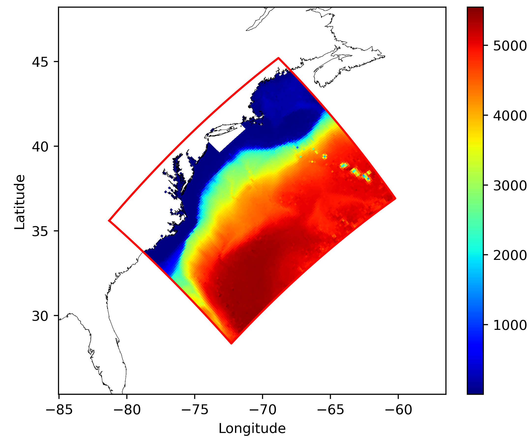
• Grid 1 (dx = 12 km, Figure 1) contains part of the U.S. East Coast from North Carolina to Maine. The domain is large enough to capture a significant amount of wind forcing from Hurricane Sandy before and immediately after landfall. The grid spacing is 12 km. Bathymetric and topographic data were extracted from the ETOPO1 global relief model with 1 arc-minute resolution (Amante et al., 2009).

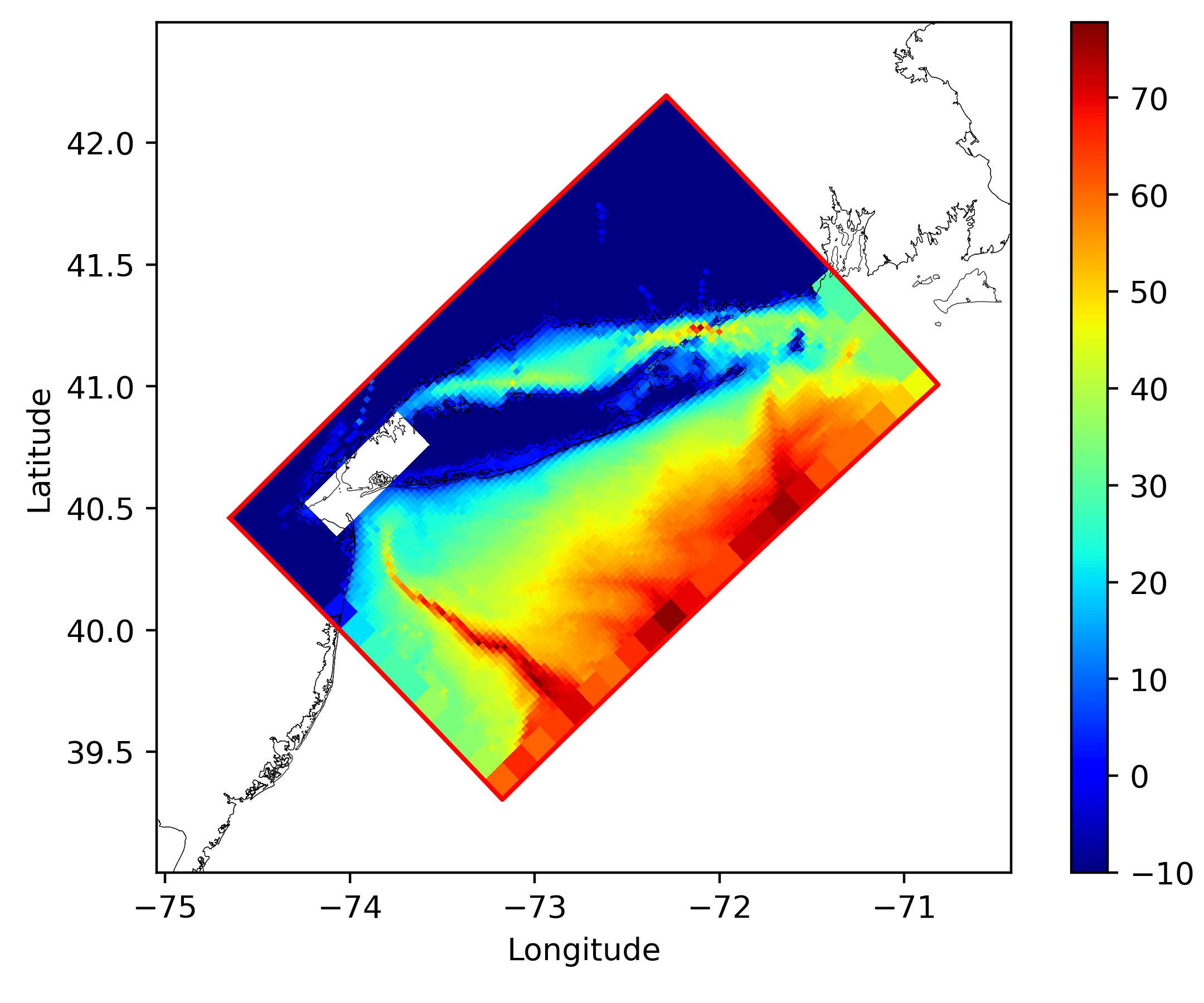
• Grid 2 (dx = 2.4 km) extends from the northern New Jersey coast to Rhode Island. Our intention in defining this grid is to transition wind and tidal forcing from Grid 1 into the coastal regions of New York Bay and Long Island Sound. The grid spacing is 2.4 km and obtained from ETOPO1.

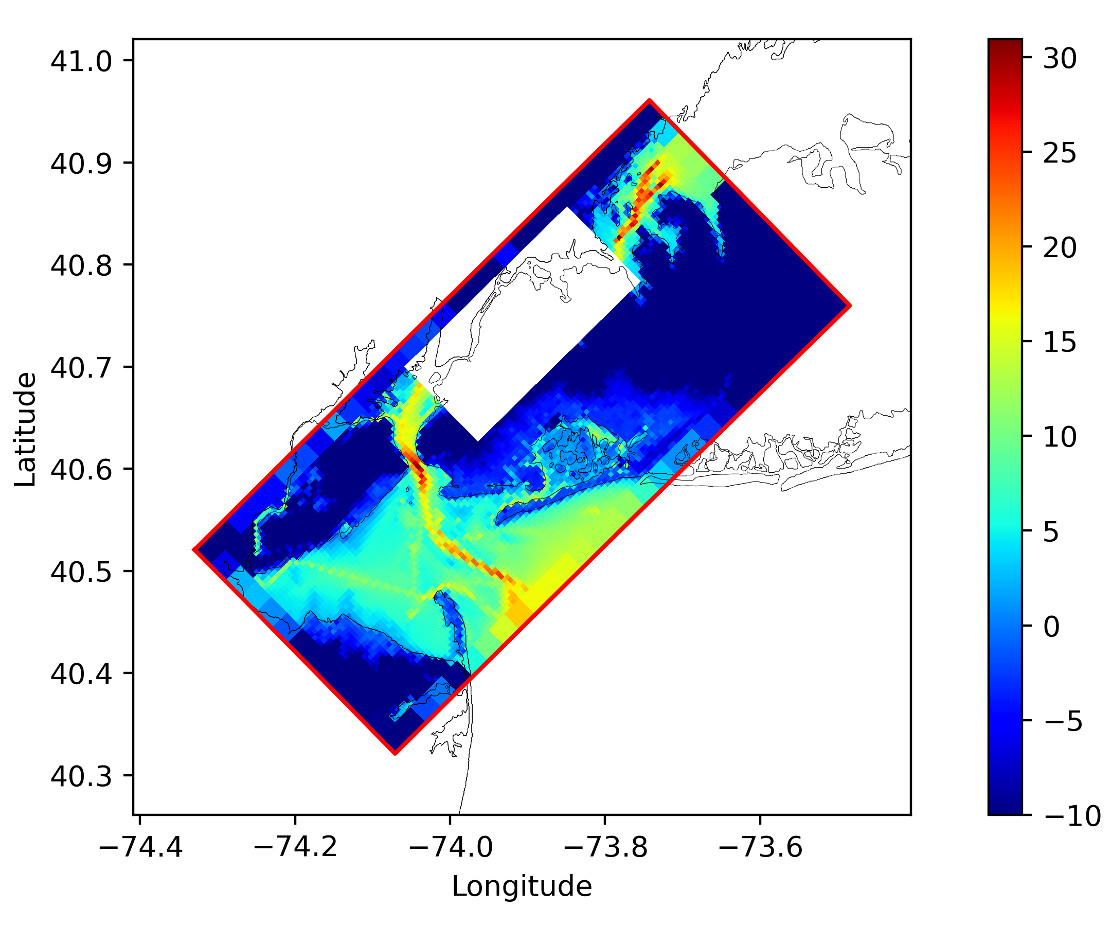
• Grid 3 (dx = 480 m) contains New York Bay and the southern end of Long Island Sound. The grid spacing is 480 m and we use data from the Continuously Updated Digital Elevation Model (CUDEM) - 1/9 Arc-Second Resolution Bathymetric-Topographic Tiles (NCEI, 2014).

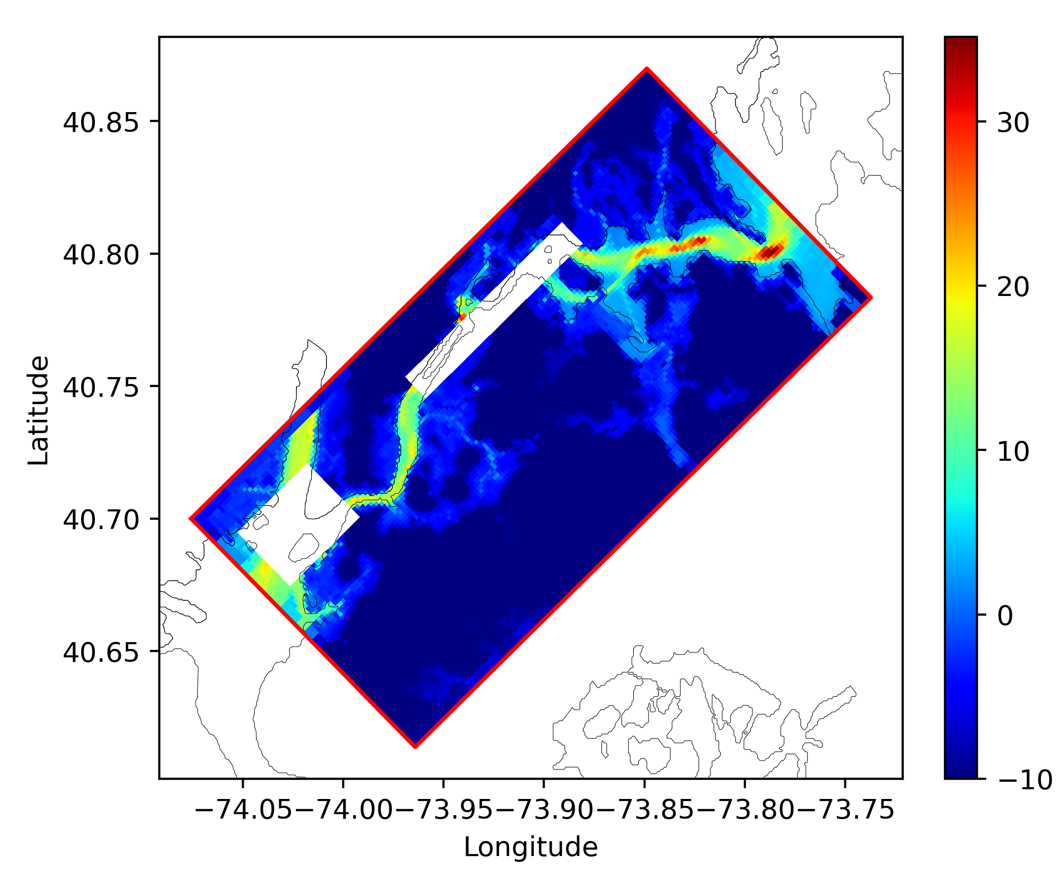
• Grid 4 (dx = 160 m) ranges from Upper Bay New York to the entrance of the East River in Long Island Sound. This grid contains the East River and the southern tip of Manhattan Island.

• Grid 5 (dx = 32 m) is placed around the confluence of the Hudson and East Rivers. Importantly for validation purposes, it contains the location of NOAA's tide gauge at the Battery .

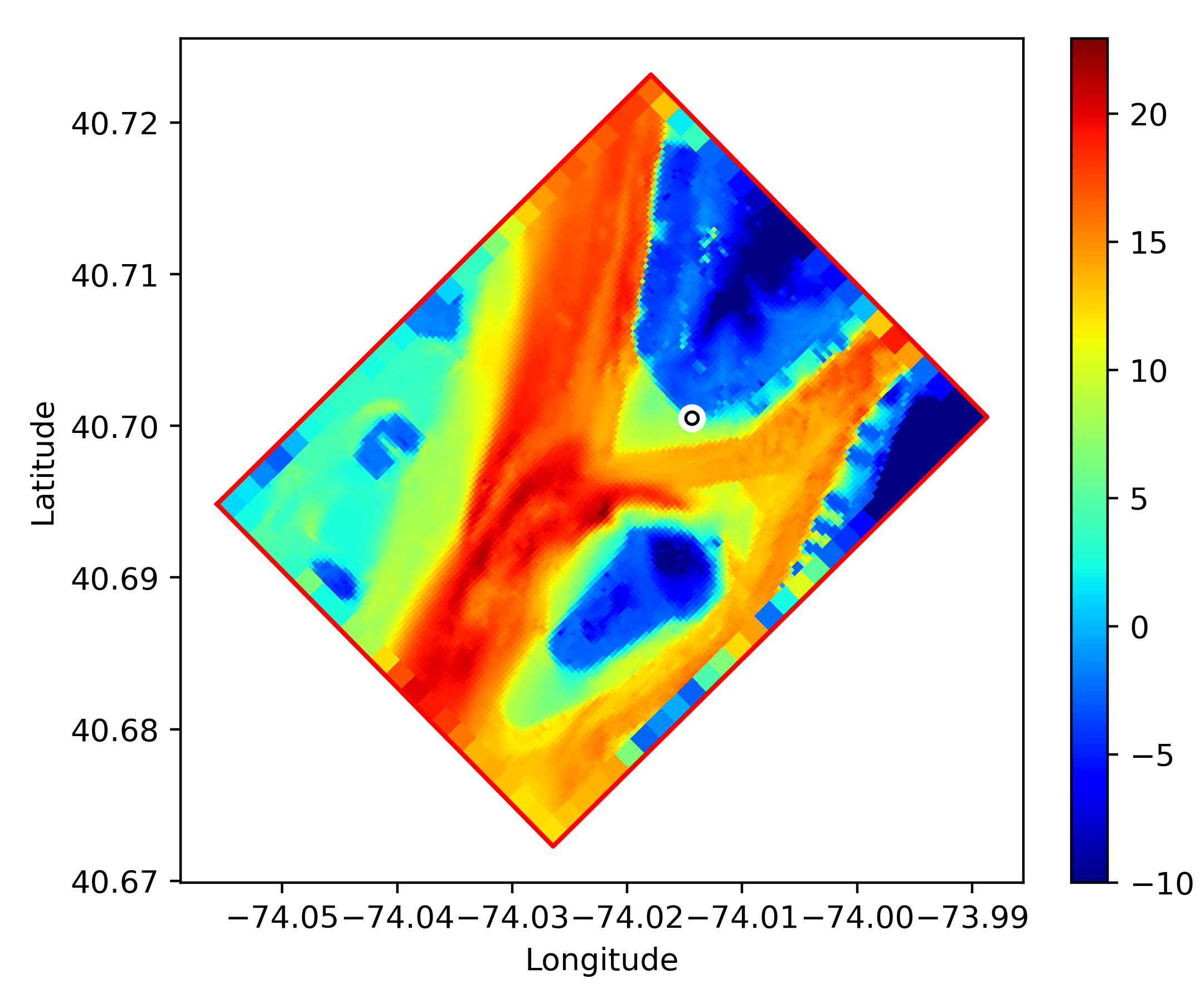
• Grid 6 (dx = 32 m) resolves the some narrow parts of the East River and extends from south of Roosevelt Island northeastwards to Rikers Island.

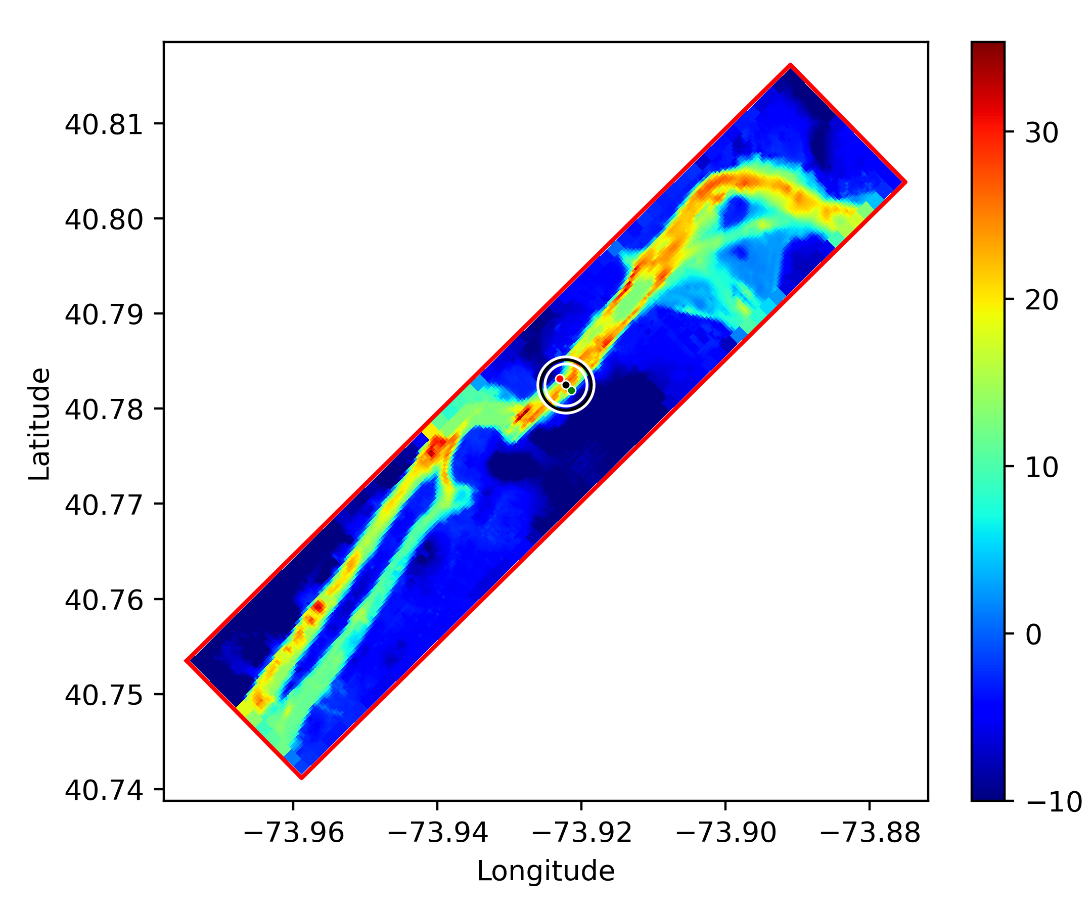
The edges of the grids cut through the Hudson and/or Harlem rivers, which are essentially both masked in this application. The effect on tidal flow and surge heights remains unknown. For the preliminary toy model described here, the goal was to resolve tidal flow through the East River at least in a qualitatively physically reasonable manner, and it is shown below that the grids are good enough for this purpose. All grids have been modified at certain grid points to avoid numerical instabilities.

ROMS supports wetting and drying of land in three-dimensional setups capability of ROMS (Warner et al., 2013). However, wetting/drying in two-dimensional setups does not work using the revision of the Rutgers code considered here. Here we use the Rutgers version of ROMS source code, specifically a revision from October 2019 (the one labeled src:ticket:826 in the version control systems). So far we know of two configuration features that conflict with wetting/drying in 2-d setups: First, the parameterization of unresolved wind-wave effects , which is not considered here, and second, grid nesting. Links to relevant forum posts are e.g. here and here .

We attempt to enable grid nesting in 2-d applications by making the following modifications:

• The array bounds in the file wetdry.F are updated to include any contact regions.
• New masks for ubar and vbar are used to exchange data between the fine and coarse grid in both direction. The masks are populated in step2d_LF_AM3.h, and simply store the coefficient cff7 used to mask u/vbar in step2d_LF_AM3.h. The new masks are submitted as arguments to the function fine2coarse2d(), instead of the previous u/vmask_full. In other words, binary masks are now submitted to fine2coarse2d() instead of the multi-valued masks that contain information about adjacent cells. The latter are used to compute the flux inhibitor for wetting/drying (Warner et al., 2013). The new masks also serve for the computation of the interpolation weights used in populating the child grid with parent grid information.
• We don't apply interpolation onto the coarse grid where the coarse grid is dry.
• The child grids are forced at the boundary with the instantaneous barotropic volume flux of the parent grid. In contrast, in 3-d setups the average over barotropic time-stepping is used. For 3-d setups, there is a CPP switch TIME_INTERP_FLUX, which linearly interpolates two bounding parent grid averages, which were previously stored after parent grid time-stepping. In this preliminary test, we omit linear interpolation in time and simply impose the most recent volume flux. Note that this may be inconsistent with the spatio-temporal interpolation of u/vbar and zeta in the remaining parts of the contact region. Further study of possible effects is deferred to future work.

These modifications were sufficient to yield reasonable results in the present setup, but are causing some instabilities in our setups.

We perform 4 experiments. Experiment TIDEONLY is forced by tidal elevation from the ADCIRC database, with ROMS' reduced physics option for tidal velocity. Experiment TIDEONLY_VEL is forced by tidal elevation and tidal velocity from the ADCIRC database. Experiment WIND is forced like TIDEONLY plus surface wind stress obtained from NCEP-NAM. Experiment WINDSTRONG is forced like WIND, but with an increased wind drag coefficient.

5.1 Tides only

Figure 12 shows results from TIDEONLY and TIDEONLY_VEL. In both experiments we use 10 tidal harmonic constitutents: M2, S2, N2, K2, K1, O1, P1, Q1, M4 and M6. Phase and amplitude of the tidal elevation at the Battery are resolved well in both cases. This is our first modeling study with tidal flow, and Appendix A provides some evidence that we are using the ADCIRC database and the T_Tide (Pawlowicz et al., 2002) library in a sensible way.

The dashed lines in figures 8 and 9 show model velocity time series in the East River (Grid 6) for experiment TIDEONLY, measured at the stations marked in Figure 6. For comparison, the solid lines show velocity extracted from the ADCIRC database.

The phase is captured well, but the amplitudes are generally smaller in our model. Sensitivity studies with respect to horizontal resolution, turbulent diffusion and bottom friction have not been conducted in this study. However, the results raise confidence that the modifications of the ROMS code regarding the barotropic velocity forcing at the boundary are sensible.

5.2 Tides and wind

Now we additionally force the model with NCEP-NAM wind, using the simple parameterization

$$\tau = C_du^2,$$

where \(\tau\) is the kinematic wind stress, \(C_d=3\cdot 10^{-6}\) is the drag coefficient and \(u\) is the wind velocity at 10 m height. Figure 10 shows observed and modelled sea surface height at the Battery during hurricane Sandy. The solid black line shows results from experiment WIND.

The model underestimates the peak surge by more than a meter. This agrees, at least qualitatively, with work by other authors (e.g. Georgas et al., 2014) who have used NCEP-NAM as wind forcing. Clearly, the simple parameterization for wind stress used here limits the significance of comparisons to recently published studies. We hypothesize the underestimation is in part due to the fact that NCEP-NAM has relatively coarse-resolution and seems to underestimate the observed wind speed in some coastal areas such as Long Island Sound (see the time series plots for station 44022 and station 44040 in one of our previous posts) and possibly other regions within New York Bay. This issue is of course very interesting from a scientific perspective. For the purpose of this blog post, however, whose simple objective is a test of ROMS' inundation capabilities, all we do is put on record that the wind forcing is too weak to create extensive inundation of the modelled regions.

To overcome this issue, we set up another experiment and simply increase the drag coefficient for wind stress by a factor of two. The resulting time series of sea surface height at the Batter is shown in Figure 10. It reproduces the observed peak surge more accurately. Note that both WIND and WINDSTRONG terminate the simulation early (as can be seen in Figure 10) due to numerical instabilities. For the purpose of this blog post, we have not investigated this issue further.

5.3 Inundation

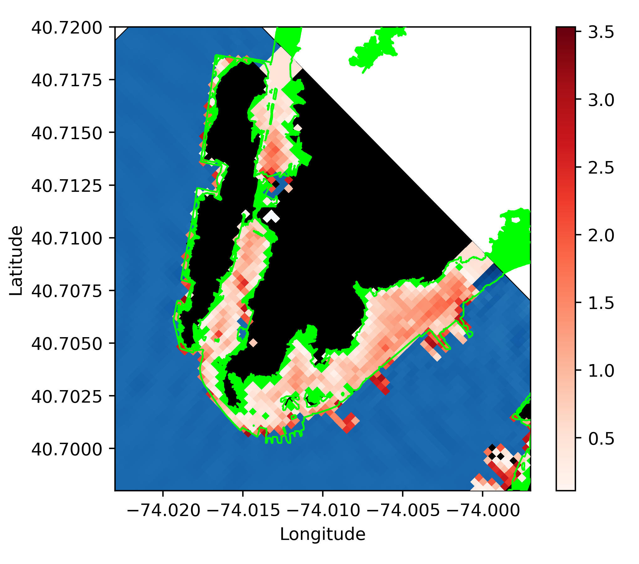
Figure 11 shows inundated regions of Grid 5. The model reproduces the observed inundation well. Several small blue patches are visible over land, which are artifacts of our model initialization procedure. These areas lie below sea level and are therefore characterized as "ocean" during initialization.

Data was provided by NOAA. NYC OpenData was provided by the Department of Small Business Services (SBS). Open source software used includes Matplotlib , PROJ , T_Tide , GNU Octave , netcdf4-python and Zhigang Xu's tidal_ellipse MATLAB tools, translated to Python by Pierre Cazenave. Other data sources and software have been cited in the main text.

The experiments described here are the author's first modeling study with resolved tidal flow. Here are some notes on how we proceeded. If you find any errors, please contact us.

7.1 Obtaining the equilibrium argument and nodal amplitude correction

First we need to obtain astronomical phase, nodal phase modulation, and nodal amplitude correction. We use the T_Tide (Pawlowicz et al., 2002) package for this purpose. Since this is our first use of this package, and since we adapted it to run under Octave instead of MATLAB, it is prudent to conduct a "sanity check" before proceeding any further. 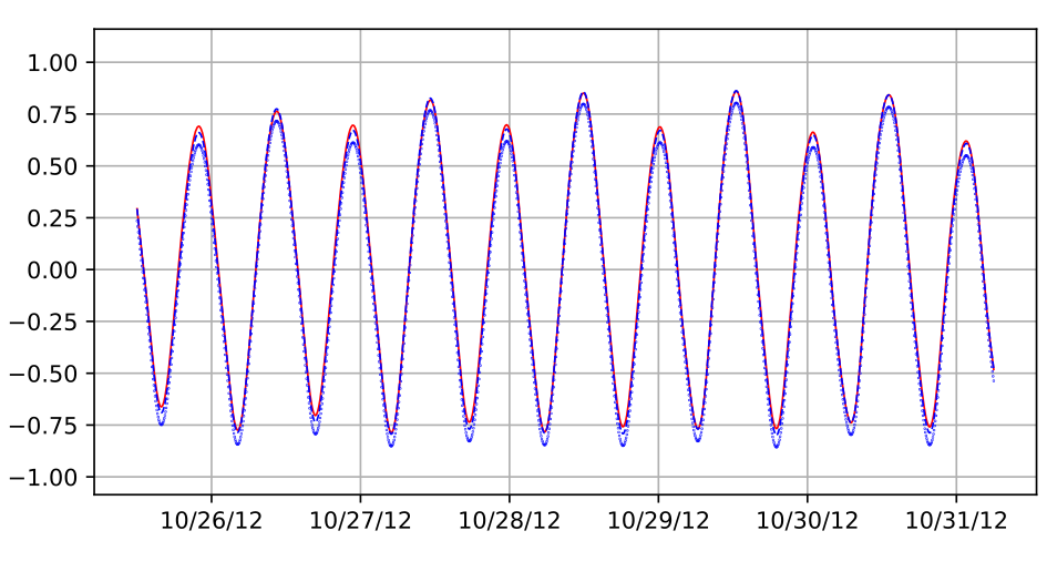Figure 12 shows a time series of predicted tidal elevation at the Battery tide gauge, retrieved from the CO-OPS API For Data Retrieval (see the station home page here ). We interpret the red line in this figure as "truth" against which we validate our approach. It does not contain any computations performed by us, but is the "official" tide prediction distributed by NOAA.

NOAA provides a description of how this type of time series is computed. To evalute the formula

$$h = Ho + \sum{fH \cos{(at + (Vo+u) - K)}},$$

or equivalently

$$h = Ho + \sum{fH \cos{(at - (K - Vo - u))}},$$

NOAA provides all variables , except the equilibrium argument \((Vo + u)\) and the nodal amplitude correction \(f\) (which dependent on the chosen origin of the time lag axis). We use the T_Tide package to compute these values for our starting date/time October 25, 12:00, and using the results we plot the blue line in Figure 12. Visual inspection suggests that we use T_Tide in a way that is sensible enough for our purposes.

7.2 The effect of using only 10 tidal harmonic constituents

Figure 13 shows the effect of using only 10 instead of 37 components. The difference is negligible for our purposes.

7.3 The effect of using phase and amplitude from the ADCIRC database

Along the boundaries of the model tidal information is retrieved from the ADCIRC database. To get a first impression about the correspondence of this database to observed values (described in detail by Szpilka et al., 2016) , we retrieve phase and amplitude around (within hundred meters of) the location of the Battery tide gauge.

References

• Amante, C., Eakins, B.W., 2009: ETOPO1 1 Arc-Minute Global Relief Model: Procedures, Data Sources and Analysis. NOAA Technical Memorandum NESDIS NGDC-24.
• Forbes, C., Rhome, J., Mattocks, C., Taylor, A., 2014: Predicting the storm surge threat of Hurricane Sandy with the National Weather Service SLOSH model
• Georgas, N., Orton, P., Blumberg, A., Cohen, L., Zarrilli, D., Yin, L., 2014: The impact of tidal phase on Hurricane Sandy's flooding around New York City and Long Island Sound.
• Lin, N., Emanuel, K.A., Smith, J.A., Vanmarcke, E., 2010: Risk assessment of hurricane storm surge for New York City
• Marsooli, R., Orton, P.M., Mellor, G., Georgas, N., Blumberg, A.F., 2017: A coupled circulation–wave model for numerical simulation of storm tides and waves.
• Mooney, P.A., Gill, D.O., Mulligan, F.J., Bruyère, C.L., 2016: Hurricane simulation using different representations of atmosphere–ocean interaction: the case of Irene (2011).
• Mooney, P.A., Mulligan, F.J., Bruyère, C.L., Parker, C.L., Gill, D.O., 2019: Investigating the performance of coupled WRF-ROMS simulations of Hurricane Irene (2011) in a regional climate modeling framework.
• NOAA National Centers for Environmental Information, 2014: Continuously Updated Digital Elevation Model (CUDEM) - 1/9 Arc-Second Resolution Bathymetric-Topographic Tiles.
• Olabarrieta, M., Warner, J.C., Armstrong, B., Zambon, J.B., He, R., 2012: Ocean–atmosphere dynamics during Hurricane Ida and Nor’Ida: An application of the coupled ocean–atmosphere–wave–sediment transport (COAWST) modeling system.
• Pawlowicz, R., Beardsley, B., Lentz, S., 2002: Classical tidal harmonic analysis including error estimates in MATLAB using T_TIDE.
• Shchepetkin, A.F., McWilliams, J.C., 2005: The regional oceanic modeling system (ROMS): a split-explicit, free-surface, topography-following-coordinate oceanic model
• Szpilka, C., Dresback, K., Kolar, R., Feyen, J., Wang, J., 2016: Improvements for the western north atlantic, caribbean and gulf of mexico adcirc tidal database (EC2015).
• Taflanidis, A.A., Kennedy, A.B., Westerink, J.J., Smith, J., Cheung, K.F., Hope M., Tanaka, S., 2013: Rapid assessment of wave and surge risk during landfalling hurricanes: probabilistic approach
• Warner, J.C., Defne, Z., Haas, K., Arango, H.G., 2013: A wetting and drying scheme for ROMS.
• Warner, J.C., Schwab, W.C., List, J.H., Safak, I., Liste, M.,, Baldwin, W., 2017: Inner-shelf ocean dynamics and seafloor morphologic changes during Hurricane Sandy.
• Westerink, J.J., Feyen, J.C., Atkinson, J.H., Roberts, H.J., Kubatko E.J., Luettich, R.A., Dawson, C., Powell, M.D., Dunion, J.P., Pourtuheri, H., 2008: A basin‐ to channel‐scale unstructured grid hurricane storm surge model applied to southern Louisiana.
• Xu, K., Mickey, R.C., Chen, Q., Harris, C.K., Hetland, R.D., Hu, K., Wang, J., 2016: Shelf sediment transport during hurricanes Katrina and Rita.