A simplistic "operational" toy model of the northern Bay of Bengal

The Regional Ocean Modeling System (ROMS, Shchepetkin and McWilliams, 2005), is a free-surface, terrain-following, primitive equations ocean model. The terrain-following coordinate system is advantageous for resolving surface and bottom boundary layers in application domains with highly variable depths, typically ranging from the deep ocean to the continental shelf. ROMS features various implementations of 4-dimensional variational data assimilation (4D-Var). The lateral grid is shown in Figure 1 and consists of 157x92 points with a resolution of about 8 km, which is only slightly higher than the parent model's resolution (about 9.2 km in meridional and 8.7 km in zonal direction, as discussed below).

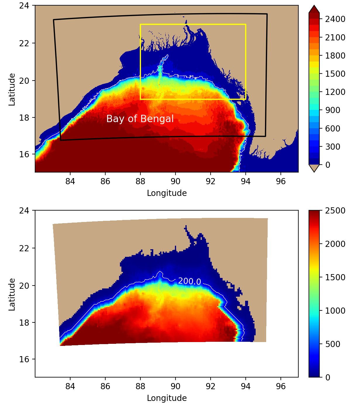
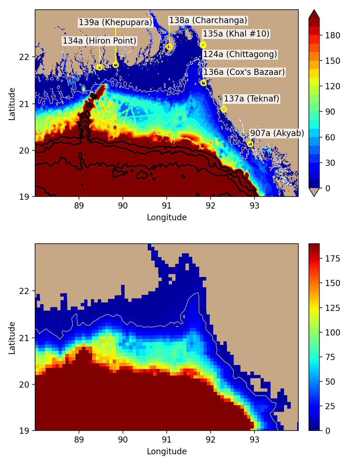
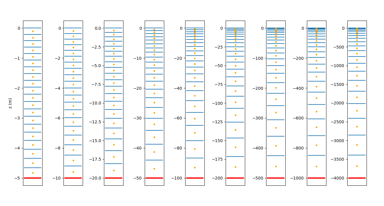
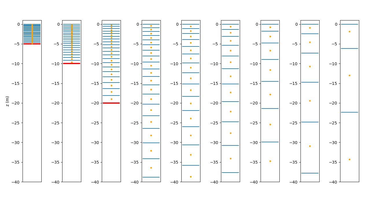
The vertical grid consists of 20 terrain-following levels. The minimum depth is set to about 5.64 m. Figure 3 shows the distribution of the vertical grid for various depths. At the present stage of model configuration, the choice of the stretching parameters for the ROMS vertical coordinate is rather uninformed. We use quadratic bottom friction, with a friction coefficient computed from an assumed logarithmic layer velocity using a bottom roughness length of 0.002 m. The choice of bottom roughness is again mostly uninformed, although based on a suggestion by John Warner in the ROMS user forum regarding tide modelling. Whether this is actually reasonable for the coarse lateral grid and the vertical grid used in our study, is currently unclear. In the following paragraph we take some notes from the literature, as a starting point for future work on this topic.

The parameterization is based on the assumption that there is a logarithmic layer (also called overlap layer or inertial sublayer), where scaling considerations for both the large-scale flow in the outer Ekman layer, and the small-scale flow in the inner Ekman layer, which is nearer to the bottom, must be valid simultaneously. This layer covers the top of the inner layer and the bottom of the outer Ekman layer (Blackadar and Tennekes, 1968). Using the terminology of non-dimensional universal laws, the velocity profile in the logarithmic layer obeys both a law of the wall (here for dynamically rough flow) and a velocity defect law (e.g. Southard, 2019). If the bottom stress points in zonal direction \((\tau_b=\tau_{bx}\)), the zonal velocity component in the inertial sublayer, i.e. for \(z_0 \ll z \ll \delta\), can be written both as

and

where \(z\) is the vertical coordinate, \(u\) is the horizontal velocity component in zonal direction, \(u_g\) is the external geostrophic velocity in zonal direction, \(u_*=\sqrt{\tau_{b}/\rho}\) is the friction velocity, \(\kappa\approx 0.4\) is the von Kármán constant and \(A\) is a constant (Grant and Madsen, 1986). The variable \(z_0\) represents the roughness length, which is often assumed to be \(d/30\) if \(d\) is representative for the mean particle size of a planar sediment layer (Southard, 2019). The quantity \(\delta=u_*/f\), where \(f\) is the Coriolis frequency, is referred to as the scale height of the Ekman layer, at least in atmospheric literature (Blackadar and Tennekes, 1968), or the overall boundary layer scale (Grant and Madsen, 1986). The above theory assumes no stratification within the planetary boundary layer, horizontally homogeneous flow with simple bottom topography and a water depth that is larger than the depth of the boundary layer. The use of \(\kappa\) in the above formulae assumes very large surface Rossby numbers \(G/(fz_0)\), where \(G=\sqrt{u_g^2+v_g^2}\) is the magnitude of the geostrophic velocity (Grant and Madsen, 1986). The actual depth of the Ekman layer is taken as \(\delta/4\) by Blackadar and Tennekes (1968) and as \(0.4\delta\) by Grant and Madsen (1986). According to Grant and Madsen (1986), laboratory studies indicate a thickness of the logarithmic layer of about 10% of the boundary layer thickness, i.e. \(0.04\delta\).

Using the notation of the ROMS wiki page about the sediment model (although we interpret \(\tau\) and \(K_M\) as dynamic instead of kinematic quantities), the vertical bottom boundary condition for horizontal velocity is written as

where \(K_M\) is the turbulent vertical viscosity and \(s\) is the vertical coordinate. To determine \(\tau_b\), ROMS provides simple drag-coefficient expressions or sophisticated bottom boundary layer parameterizations. The options for simple drag-coefficients are linear, quadratic or "logarithmic" drag. The commonly used term "logarithmic" may be somewhat misleading, since the expression for computing the stress from velocity is quadratic (see also the documentation of the croco and NEMO models). For the quadratic drag parameterization, the bottom stress magnitude is

where \(c_D\) is a nondimensional drag coefficient and \(u_N\) is the horizontal velocity at the deepest velocity grid point. Note that in the case of ROMS, the grid point is vertically centered within the layer formed by the lowest grid cells. The drag parameterization is called "logarithmic" if \(c_D\) is computed from the assumption that the velocity profile between the bottom and the lowest grid cell follows the logarithmic-layer profile, i.e.

If \(u_*=\sqrt{|\tau_b|/\rho}\),

which, according to the quadratic drag parameterization, implies a definition of \(c_D\) as

A possible advantage of the "logarithmic drag" is that it takes into account the distance between the bottom and the lowest grid point. Figure 3 shows that in our preliminary configuration, this difference varies by multiple orders of magnitude within the domain. Using a "quadratic drag" parameterization, the drag coefficient would be independent of the cell height. Figure 3 shows that the lowest cell height is roughly 150 m in depths of 1000 m, and the velocity grid point is roughly 75 m above the bottom. This distance is orders of magnitude larger than the thickness of the logarithmic layer, and may also be well above the top end of the Ekman layer. Hence, it is currently unclear to us whether the "logarithmic drag" for our grid is meaningful, and the topic requires further literature review.

Figure 2 shows that the 8 km resolution is barely able to resolve at least schematically one of the world's largest river mouth, but fails to resolve the many smaller rivers west of the major mouths and in the Sundarban region. In search for a fully automated grid manipulation method applicable to other regions of the world, we chose to average the 15 arc-second (about 450 m) GEBCO_2021 GEBCO (2021) bathymetry in bins formed by grid cells of our 8 km grid. This is done in projection space and seems to result in a connected system of river mouths without requiring manual removal of masked ("land") points, but seems to have the drawback that the resulting river mouths are generally too wide and too shallow. In the final topography, the Meghna is split into Shahbazpur Channel flowing to the west of a poorly represented Hatiya Island, and another mouth flowing to the east of the island. A minimal representation of Sandwip Island in the north-easternmost part of the domain also remains. To avoid numerical instabilities, the bathymetry is smoothed using a method similar to the one described by Martinho and Batteen (2006) with a target slope factor of 0.2, except that the factor is enforced by decreasing overly steep increases of depth, i.e. by producing shallower than observed depths (Dutour-Sikirić et al., 2009). To this end, we used the pyroms Python package (Hedstrom et al., 2020), which contains a Python translation (in the folder "bathy-smoother" of the pyroms package) of the Matlab code originally developed by Dutour-Sikirić et al. (2009). We chose to make large depths shallower (instead of the opposite) so that the wide shallow region with depths of less than 10 m surrounding the river mouths remains similar to the real bathymetry. Figures 1 and 2 show that this generally results in a widening of both shelf and slope. This may have profound effects on the circulation, although in comprehensive, large nested models with variable resolution, this issue may be less problematic.

The initial and boundary conditions for the regional model are interpolated from the Copernicus Marine Environment Monitoring Service (CMEMS) global analysis and forecast product GLOBAL_ANALYSIS_FORECAST_PHY_001_024 (link accessed December 16, 2022), here referred to as NEMO-CMEMS (Lellouche et al., 2018). Two years of forecast/analysis data up to the present time are available from the data archive linked on the CMEMS website. The documentation states that an archive of analysis since 26/12/2006 up to real-time is available on their server, but we have not accessed this extended archive. NEMO-CMEMS has 50 vertical levels and a 1/12 degree resolution, which is about 9.2 (8.7) km in meridional (zonal) direction at a latitude of 20 degrees north. It is forced atmospherically with 3-hourly ECMWF fields and uses a data assimilation scheme ingesting sea ice concentration data, sea level anomaly and temperature data measured by satellite altimeters, in-situ profiles of active tracers and a temperature/salinity climatology below 2000 m. The bathymetry is composed of interpolated ETOPO1 (Amante et al., 2009) and GEBCO8 (GEBCO, 2008) data sets. NEMO-CMEMS provides daily 10-day forecasts and weekly assimilation analyses.

NEMO-CMEMS does not simulate tides or atmospheric pressure effects. For comparison of simulated sea level data to observed tide gauge data, a set of GLOSS/CLIVAR (link accessed November 16, 2022) instruments have been filtered to correct for inverse barometer effect and tides Lellouche et al. (2018, their section 4.3.2). High-frequency model SSH compares well with tide gauges in many places and Lellouche et al. (2018) state that the agreement is best in the tropical band, while shelf regions and closed seas are less accurate.

The scheduling of analysis and forecast runs is depicted in the product user manual (link accessed 2022/11/23). The model is run daily with updated atmospheric forcing fields, without assimilation, for days D-1 to D+9 (one day before present time to 9 days after present time), starting from the end of D-2. Once every week (on Wednesdays), the model is run with assimilation for days D-14 to D-1. Solutions for days D-14 to D-8 constitute the "best analysis" and for days D-7 to D-1 the "analysis". In our "operational" toy model we use 6 days, i.e. days D-3 to D+2 for lateral boundary conditions. One issue we encountered is that once every week after the assimilation run of NEMO-CMEMS, the boundary conditions seem to contain discontinuities with respect to the previous day, causing significant spurious oscillations of the free surface, which propagate towards the coast and affect the coastal water level. This issue may be resolved by (1) starting our model once a week on D-14 in synchronization with the NEMO-CMEMS assimilation, or (2) by modifying our boundary conditions to dampen the barotropic effects of the discontinuities. This is beyond the scope of this note.

Although the author of this note has no prior experience with data assimilation, we try to summarize some points of Lellouche et al. (2018) that seem relevant in the context of sea level modelling in general. NEMO-CMEMS uses the Boussinesq approximation, and the equations of motion conserve volume instead of mass. According to Lellouche et al. (2018), this is problematic when assimilating altimetry data, because the altimeters are affected by long-term sea level rise and this trend is not filtered from the altimeter data. NEMO-CMEMS therefore contains two additional parameterizations to induce an estimate of sea level rise in order to improve consistency with assimilated altimetry data. However, Lellouche et al. (2018) also state (on their p. 1100) that the altimetry data and the in-situ profiles of temperature and salinity are insufficient to control the modelled mean sea level by assimilation. Therefore, the global mean increment of the total sea surface height is set to zero (we assume the term "increment" is used in their article as a technical term for the "correction induced by the assimilation procedure"). The two additional parameterizations to artificially incude a sea level rise are as follows: First, a time-evolving global mean steric effect is added to the modelled sea level. Second, a trend of 2.2 mm yr-1 is added to the surface mass/volume budget which represents an estimate of the global mass addition to the ocean from glaciers, land water storage changes and ice sheet mass loss. This term is implemented as a surface freshwater flux in the open ocean in regions with many icebergs. Furthermore, since uncertainties in the water budget closure can cause a drift in the sea surface on longer time scales, the surface freshwater global budget is set to an imposed seasonal cycle.

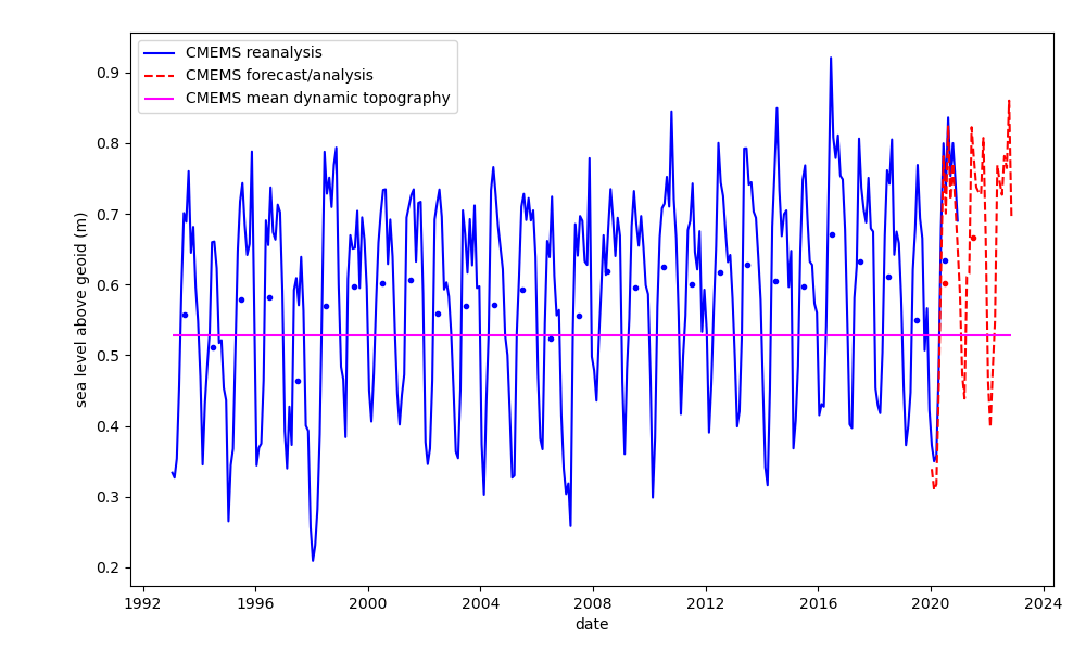
Both the NEMO-CMEMS analysis/forecast and reanalysis datasets contain a mean dynamic topography (mdt) field, which is described as sea surface height above geoid and measured in units of meters. One particular aspect of NEMO-CMEMS we do not currently understand, is how to interpret mean sea level anomaly with respect to this mdt field. When plotting the mean sea level anomaly of NEMO-CMEMS with respect to the two previous years, i.e. the difference between the mean monthly zos variable (which is also described as sea surface height above geoid), and the mdt field (mean dynamic topography) in the Bay of Bengal for the two years before present, there is a mean difference on the order of 10 cm. This difference seems large, and its origin is currently unclear to us. However, we hypothesize that the mdt fields may be representative for the early 1990s, such that the offset could be the result of continuous artificial mean sea level corrections described above, applied over 3 decades. We have not yet fully understood the article of Lellouche et al. (2021), which may resolve the issue. For now, we can plot Figure 5 showing the monthly mean sea level extracted from both the CMEMS reanalysis and forecast/analysis data sets. The sea level is extracted at the Chattogram tide gauge. For a plot of the monthly-mean global-mean sea level, see Fig. 14 of Lellouche et al. (2021). The figures seem consistent with the hypothesis that the mdt field represents the state of the ocean surface in the early 1990s. Note that in the context of this study, this issue may not be critical, because the longest time interval under consideration is less than 3 years. However, it is instructive to keep the issue in mind when looking at plots of sea level anomaly of the NEMO-CMEMS model shown below, since we define this anomaly with respect to the mdt field, and the offset of unknown origin is clearly visible in the figures.

The Global Forecast System (GFS) provides atmospheric forcing fields at 0.25 degrees resolution. For the "operational" version of the toy model we use three-hourly fields from the NOAA Operational Model Archive and Distribution System (NOMADS) . At the time of writing, the GFS major version number used at NOMADS is 16. In this preliminary study, we treat the atmospheric model and the bulk fluxes parameterizations for surface stress and heat/salt flux mostly as a "black boxes". The only validation is done indirectly via assessment of the generated water level time series, and given the importance of atmospheric forcing for storm surge simulations, this is perhaps the most important shortcoming of the progress presented here. For the multi-year experiment, we use NCEP FNL (Final) operational global analysis and forecast data from the Global Data Assimilation System (GDAS) (RDA NCAR, 2015). The difference between GFS and FNL is explained in a blog post by NCAR (accessed November 16, 2022). FNL and GFS are related in that both systems use the same data assimilation and forecast system. However, the FNL final analysis is slightly delayed, and typically ingests about 10% more observations than GFS.

To compute surface stress and net heat/salt fluxes, we use ROMS's implementation of the parameterizations described by Fairall et al. (1996). The ROMS option EMINUSP activates a method to compute the evaporation rate from the latent heat flux and the latent heat of vaporization. We download the following fields from NOMADS or RDA-NCAR:

• wind at 10 m above surface
• pressure reduced to mean sea level
• upward/downward short wave radiation flux
• upward/downward long wave radiation flux
• temperature at 2 m above surface
• relative humidity at 2 m above surface
• precipitation rate at the surface

The performance of the FNL forcing for the multi-year experiment is compared below to the ERA5 global reanalysis (Hersbach et al., 2020). For ERA5, we compute relative humidity from the temperature and dew point temperature at 2 m height following the method suggested by John Wilkin in the ROMS user forum .

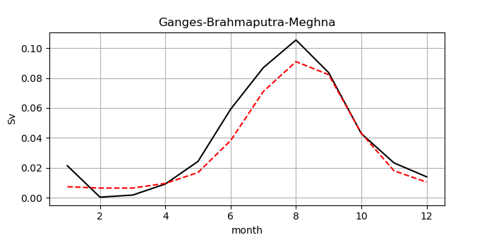
The model contains simplified forcing by freshwater discharge from the Ganges-Brahmaputra-Meghna (GBM) delta, i.e. the climatological seasonal cycle of discharge shown in Figure 6. Discharges from smaller rivers (see e.g. Jana et al. 2015) are omitted. In particular, the Karnaphuli River entering the Bay of Bengal at Chattogram (Chittagong) is not represented in the model. We have no prior experience with river forcing and our initial goal was to apply exactly the same forcing as in the NEMO-CMEMS model, ideally from a ready-to-use data set containing tables of discharges at NEMO's coastline. However, we do not know if or how this data is accessible to the public. Hence, the initial goal was abandoned in favour of the following approach, which is (1) mostly driven by the need to learn a little bit about how river discharge is computed in general, and (2) depends only on globally available dataset with global coverage. We use two sources for the calculation of the discharge. First, a definition of the geometrical shape of the Ganges-Brahmaputra-Meghna basin by Fekete et al. (2002), and second, discharge data from 1949-2004 associated with the publication of Dai and Trenberth (2002). Unfortunately, at the time of writing, the data set containing the monthly mean annual discharge cycle gridded on a 1 by 1 degree latitude/longitude grid does not seem to be accessible via the internet. The corresponding file was accessed around December 2021 from the following resource:

http://www.cgd.ucar.edu/cas/catalog/surface/dai-runoff/runoff2ocean-mon-fromStn-1deg-2d.bin

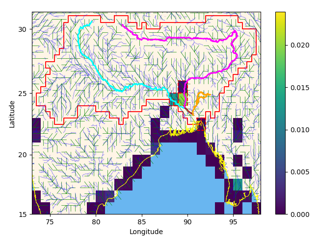
Upon inquiry, staff members of UCAR kindly informed us that the CAS Data Catalog has been retired in favor of the Climate Data Guide, and the data catalog owners have advised to reach out to Dr. Dai for references/citation purposes, or to get them added to the RDA website. We speculate that e.g. Bourdallé-Badie and Treguier (2006) refer to a similar (perhaps identical?) data set, but its role in the preparation of updated river forcing method for the NEMO-CMEMS as described by Lellouche et al. (2018) remains unclear to us. Figure 6 shows the discharge we applied at the mouth of the GBM delta at one single grid point. The application at a single grid point is an approximation. More elaborate studies apply the outflow at multiple grid points distributed in part across the Sundarban region (e.g. Jana et al., 2015). The discharge shown in Figure 6 is the sum of 4 discharge data points located within (or exactly on) the boundary of the GBM delta as defined by Fekete et al. (2002). Figure 7 shows an overview map and the 4 contributing grid points are encircled with a dashed red line. The total annual discharge from these points is 0.033 Sv. Figure 6 also shows monthly runoff data from the Simulated Topological Networks (STN-30p) Version 5.12 data of Fekete et al. (2002), integrated over the Ganges Basin (outlined by the red line in Figure 7). The data set could be accessed on November 11, 2022 at the following links:

• https://www.compositerunoff.sr.unh.edu/html/Data/index.html
• https://wsag.unh.edu/Stn-30/stn-30.html

Our values for runoff and discharge shown in Figure 6 based on the aforementioned data sets may be compared with Fig. 5a of Dai and Trenberth (2002), which shows a similar plot in the lower left panel. There, river-basin integrated precipitation is also shown. As in our figure, the pronounced annual cycle of runoff and discharge peaks in August. Dai and Trenberth (2002) states that the difference between runoff and discharge generally illustrate the effects of snow and the time delay of water traveling downstream to the river mouth, and that a relative short time lag (about 1 month or less) between the two quantities suggest that the seasonal changes in surface runoff occur in the area not far away from the river mouth. We speculate that this may be mostly driven by monsoonal rain in the area under consideration.

The regional model has an open boundary in the south, where boundary conditions for sea surface height, velocity, potential temperature and salinity are interpolated from the NEMO-CMEMS daily mean fields, which represent the solution exterior to the regional domain. For the sea surface height, hourly mean fields are available and presumably preferable, but this has not been tested in the initial study described here. For the 3d velocity and tracer fields, instantaneous fields with a temporal resolution of 6 hours are available and presumably preferable, but again this has not been tested. Inital conditions are also interpolated from the daily mean fields. No tides are simulated in this initial study.

For the boundary conditions of 3d velocity and tracers we use the ROMS implementation of an adaptive algorithm where inward and outward propagating signals are treated separately, originally developed by Marchesiello et al. (2001). External data required for inward boundary fluxes is imposed via adaptive "nudging" (relaxation). Outward fluxes are treated with an algorithm for two-dimensional radiation. The radiation condition is used to determine whether fluxes are inward or outward. In the latter case, weaker nudging prevents substantial drifts during longer periods of continuous outflow, while reducing over-specification (Marchesiello et al., 2001).

We use a nudging time scale of 2 days for inflow and 5 days for outflow, for both momentum and tracers. Furthermore, a "nudging layer" (using the terminology of Marchesiello et al., 2001) is used to relax model data in the interior towards NEMO-CMEMS data, again for both momentum and tracers. The nudging layer is limited to a region adjacent to the open boundary, where we use a nudging time scale of 5 days decreasing linearly to zero about 160 km inwards of the boundary. In the same region, a "sponge layer" is used in which turbulent viscosity and diffusivities are linearly increased from the interior value to a 10-fold of the interior value at the boundary. We have not assessed the sensitivity to these parameters, since this requires analysis of the circulation and water mass characteristics.

For the normal component of barotropic velocity, we use the boundary condition of Flather (1976) or Reid and Bodine (1968) (see note by H. Arango regarding the correct attribution)

where \(\overline{u}\) is the barotropic velocity component orthogonal to the boundary, \(\overline{u}^{ext}\) is the corresponding exterior value, \(g\) is the gravitational acceleration, \(h\) is the depth, \(\zeta\) is the free surface at the boundary, and \(\zeta^{ext}\) is the corresponding exterior value. In toy models for storm surge studies, \(\zeta^{ext}\) may be the prescribed variable, and the question arises how to obtain \(\overline{u}^{ext}\). Although the article of Flather (1976) does not seem to be available on the internet, Flather (1987) uses a similar boundary condition in a tidal model, only as the second step of a two-step procedure. The first step is to use a "clamped" boundary condition for \(\zeta\), i.e.

which they use in combination with strong friction to dampen waves generated/reflected in the interior of the domain, such that they effectively vanish before they reach the boundary, where they otherwise would be reflected by the clamped condition back into the interior and cause instabilities. Flather (1987) argues that while the strong friction degenerates the solution on the continental shelf due to the exaggerated damping in shallow water, the velocities in deep water adjacent to the boundary are not much affected. In the second step, they use these velocities from the first step as \(\overline{u}^{ext}\) in the gravity-wave radiation condition given above. We instead use the "reduced physics" approach described in Flather and Davies (1975) and the ROMS wiki (accessed November 24, 2022). The velocity at the boundary is computed as a function of (1) its present value, (2) external sea level signals, (3) the Coriolis force acting on the velocity, (4) the wind stress. If ROMS is configured to resolve sea level oscillations caused by variations in atmospheric pressure, but the parent model does not resolve them, then ROMS provides an additional option to add this component into the boundary condition. Atmospheric pressure effects are not resolved in this study. To simplify further notes on the Flather boundary condition, we additionally assume zero Coriolis force and wind stress in the following.

Eq. \eqref{eq:forum} is similar to the one given in the ROMS wiki , but using \(h\) instead of \(D\) to link to the notation of Blayo and Debreu (2005), who state in their section 3.2 that the Flather condition can be obtained by the Sommerfeld condition for the surface elevation \(\zeta\) (with surface gravity waves phase speed) and a one-dimensional approximation to the continuity equation. They consider a small-amplitude shallow water wave propagating from the interior through an eastern boundary to the exterior, i.e. the outward unit normal of the boundary is the unit vector in direction of the x-axis, and the phase speed is positive. Note that \(c/h=\sqrt{g/h}\), where \(c\) is the phase speed. Eq. (25) of Blayo and Debreu (2005) is then

Multiplying a finite difference representation of the preceding equation by \(dx\) gives

Assuming an eastern boundary, one may choose to drop the index \(i\) and label \(i+1\) as exterior (\(ext\)), yielding

At a western boundary, one may use \eqref{eq:labelled} with a different physical interpretation. Rewriting Eq. \eqref{eq:flatherfd}

labelling the point \(i\) the exterior and dropping the index \(i+1\), as appropriate for a western boundary condition, results in the same form as \eqref{eq:labelled}. However, the condition now has an active forcing character, rather than a passive absorbing one, consistent with the initial assumption that the phase speed is positive along the x-axis. Whether the "labelled" form \eqref{eq:labelled} lets outward propagating waves pass through the boundary, or force the interior with waves coming from the outside, depends on whether the phase speed points into the domain or to the outside. In a finite difference expression for a given boundary, the phase speed can be flipped by swapping the \(\zeta^{i}\) and \(\zeta^{i+1}\) terms (or the \(ext\) label) on the right hand side of the expression. For example, Eq. \eqref{eq:forum} could serve as an absorbing condition at a western boundary.

Regarding the implementation in ROMS, consider a Flather condition for a western boundary, without Coriolis force, wind stress and atmospheric pressure correction.

The corresponding FORTRAN code block ("Western edge, Flather boundary condition" in the file u2dbc_im.F) is

    
            ubar(Istr,j,kout)=bry_val-                                &
    &                          Cx*(0.5_r8*(zeta(Istr-1,j,know)+        &
    &                                      zeta(Istr  ,j,know))-       &
    &                              BOUNDARY(ng)%zeta_west(j))
    

Note that the code block may not represent a spatial gradient in any way (provided that our interpretation of the staggered location of BOUNDARY(ng)%zeta_west(j) is correct, see below). Both the average of zeta, and the term BOUNDARY(ng)%zeta_west(j) are centered at ubar points (for the centering of the latter term, see e.g. routine set_tides.F). A derivation of the radiation condition without the use of spatial gradients is given e.g. in Flather and Davies (1975). Let's denote an internally generated disturbance as \(\eta'\) and an externally generated disturbance as \(\hat{\eta}\),

In the context of their article, \(\hat{\eta}\) is an elevation associated with (quote) the externally generated [storm] surge entering the model (end quote). If we understand correctly, \(\eta\) in their article is the sea level anomaly, which is why we chose the symbol \(\eta\) instead of \(\zeta\), which in ROMS terminology is the full sea level measured from a geoid. In other words, the anomaly \(\eta\) in Eq. \eqref{eq:g1} is partitioned into two contributions, an internally and an externally generated disturbance. They introduce a condition that ensures outward propagation of the internally generated disturbance

where \(q'=q-\hat{q}\) is the associated outward going current across the boundary and \(A'\) is an appropriate admittance coefficient with dimensions of velocity. Note that they interpret \(q'\) always as the outward flux. To close the problem, \(\hat{q}\) must be specified. The option \(\hat{q}=0\) yields

Another option is to associate \(\hat{q}\) with incoming signals. Quoting Flather and Davies (1975), (quote) a radiation condition should also be applied to this incoming part of the motion (end quote), where the incoming part is storm surge energy in the context of their paper. The terminology used here is interesting, since it associates the term "radiation condition" with an actively forcing boundary condition (as opposed to a passively absorbing one). They write the condition as

where \(\hat{A}\) is another admittance coefficient and the negative sign indicates that the energy propagates inward. Using \eqref{eq:f2} in \eqref{eq:f1} yields

and setting \(A'=\hat{A}=\sqrt{gh}\) yields

To associate Eq. \eqref{eq:f1} with the ROMS code block shown above, note again that \(q\) is the outward flow, and the code block is for a western boundary. Setting

in Eq. \eqref{eq:f1} yields

leaving the difference between zeta at time know and the boundary value to be interpreted as \(\eta'\). The term \(\overline{u}^{ext}\) (bry_val) is computed in ROMS as follows (we assume zero Coriolis force, wind stress and atmospheric pressure correction)

    
              bry_pgr=-g*(zeta(Istr,j,know)-                            &
     &                      BOUNDARY(ng)%zeta_west(j))*                 &
     &                  0.5_r8*GRID(ng)%pm(Istr,j)
              Cx=1.0_r8/SQRT(g*0.5_r8*(GRID(ng)%h(Istr-1,j)+            &
     &                                 zeta(Istr-1,j,know)+             &
     &                                 GRID(ng)%h(Istr  ,j)+            &
     &                                 zeta(Istr  ,j,know)))
              cff2=GRID(ng)%om_u(Istr,j)*Cx
              bry_val=ubar(Istr+1,j,know)+                              &
     &                cff2*bry_pgr
     

Substituting the value for bry_pgr, the last line can be rewritten as

    
              bry_val=ubar(Istr+1,j,know)-                              &
     &                cff2*g*(zeta(Istr,j,know)-                        &
     &                      BOUNDARY(ng)%zeta_west(j))*                 &
     &                  0.5_r8*GRID(ng)%pm(Istr,j)
    

To get rid of the grid increment term GRID(ng)%om_u(Istr,j) and the inverse grid increment GRID(ng)%pm(Istr,j), let's assume the \(\xi\)-axis of the grid points eastward and the spacing is equidistant. Then

The term Cx represents

where \(D\) is the bottom depth, which we loosely interpret as \(h\) such that g*Cx represents \(\sqrt{g/h}\). Rewriting the code block informally with these continuous expressions,

    
              bry_val=ubar(Istr+1,j,know)-                              &
     &                sqrt(g/h)*(zeta(Istr,j,know)-                     &
     &                      BOUNDARY(ng)%zeta_west(j))*                 &
     &                  0.5_r8
     

The term bry_val seems to be centered at the "physical" western boundary of the grid, i.e. at u-points. This is supported by the first code block shown above, where bry_val is added to ubar(Istr,j,kout). Hence the preceding code block looks similar to a finite difference representation of Eq. \eqref{eq:flatherfd}, i.e.

which, as noted above, has an active forcing character at western boundaries. In the ROMS user forum, the significance of the factor 0.5 in the preceding code block was discussed. Some users argued that the term zeta(Istr,j,know)-BOUNDARY(ng)%zeta_west(j) represents a difference between two grid locations that are separated by half a grid increment, which would suggest the use of a factor 2 instead of 0.5 in the preceding code blocks (note that \(1/(0.5dx)=2/dx\)). This interpretation is supported by a comment in the file set_tides.F:

    
!  If appropriate, load tidal forcing into boundary arrays.  The "zeta"
!  boundary arrays are important for the Flather or reduced physics
!  boundary conditions for 2D momentum. To avoid having two boundary
!  points for these arrays, the values of "zeta_west" and "zeta_east"
!  are averaged at u-points.  Similarly, the values of "zeta_south"
!  and "zeta_north" is averaged at v-points. Noticed that these
!  arrays are also used for the clamped conditions for free-surface.
!  This averaging is less important for that type ob boundary
!  conditions.
     

If you know which factor should best be applied, kindly let me know. Hernan Arango pointed out in the ROMS user forum that it's a matter of testing. He also pointed out that \(u^{ext}\) should include tidal currents. We will test this in the near future.

Sea level data from a tide gauge in Chattogram (Chittagong) was obtained from the IOC sea level monitoring facility maintained by the Flanders Marine Institute (IOC/VLIZ, 2022). For each instrument on the tide gauge (pressure sensor, radars, float with encoder), we apply spike-removal, flatline-removal, interpolation, regridding and filtering procedures to the IOC time series. The data is then sub-sampled hourly and, if the quality of the resulting hourly time series permits, undergoes harmonic analysis. Using the tide prediction based on harmonic analysis, we construct a "de-tided" series by applying a low-pass filter to cut off signals in the diurnal band or higher. The steps are described in more detail below. Although we attempt to follow standard procedures for handling tide gauge data ( IOC 2020; IOOS 2021; Caldwell 2015), more research is necessary to ascertain that we follow currently accepted best practices at each of the following steps.

1. Spike removal. Values deviating from the mean more than three times the standard deviation are removed from the time series.
2. "Flatline" removal. Consecutive values with identical sea level value are removed.
3. Interpolation to 5 min. The time series is re-gridded onto a 5-minute time axis using cubic splines with low smoothing. Data points isolated by 10 minutes or more from their neighbours are discarded before the interpolation.
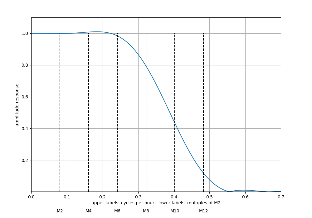
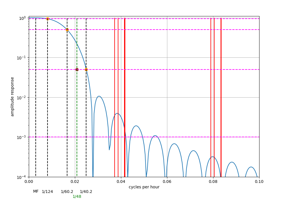
4. Digital low-pass filter 1. To obtain hourly values free of aliased high-frequency signals, we apply the filter described by (Pugh, 1987) for a sampling rate of 5 minutes. The frequency response of the filter is shown in Figure 8. Somewhat suspiciously, it is not exactly identical to the response shown in figure A1:1 of (Pugh, 1987). Our figure shows an overshoot between M2 and M6, and a side lobe at the right end of the axis. Both features are not visible in Pugh's plot. They may result from a processing error on our part and further work on digital filters is required.
5. Subsampling of hourly values. The filtered 5-minute series is subsampled by collecting all values that occur at full hours.

Based on the quality of the resulting hourly time series for each instrument, we choose the time series which is most complete and/or contains the least number of suspicious looking signals (indicating possible instrument errors) to perform harmonic analysis. We aim to process 366 days of valid data in the harmonic analysis. Since the hourly series usually do not yield contiguous intervals of an entire year, the data is scattered in discontinuous patches among multiple years, sometimes with gaps of weeks or months filled with invalid data. We use the UTide harmonic analysis method of (Codiga, 2011) developed for irregularly distributed time series, in the form of W. Bowman's UTide Python software package. Using the harmonic constants, we construct a residual time series by subtracting diurnal and higher-frequency tidal signals from the original hourly series. Finally, a "daily" time series is obtained by filtering the residual with a digital filter extracted from the SLP64 software package distributed by the University of Hawaii Sea Level Center (Caldwell, 2015). To summarize, we take the following steps.

6. Harmonic analysis. The hourly time series is processed with the UTide harmonic analysis method.
7. Hourly residual. A residual time series is formed by subtracting constituents with diurnal or higher frequencies from the hourly series. Note that constituents with periods longer than diurnal are still present in the residual.
8. Digital low-pass filter 2. The residual time series is filtered using a filter shape copied from the file FILTHR.FOR of the SLP64 package, representing a 119-point convolution filter according to Caldwell (2015). The resulting time series may be interpreted to represent "daily averaged" data. Throughout this blog post, we refer to this time series as SLA-LPF (low-pass filtered sea level anomaly)

Note that our low-pass residual is computed differently than the analogous residual used in the SLP64 package, where only four dominant tidal components (M2, S2, K1, and O1) are removed from the hourly series (see subroutine Calres in the file FILTHR.FOR in the SLP64 package). We have not quantified the difference between the methods. The frequency response of the low-pass filter is shown in Figure 9. Somewhat suspiciously, it is partly inconsistent with the response described in Caldwell (2015). In their section 6.1, they state that

The 95, 50, and 5% amplitude points are 124.0, 60.2, and 40.2 hours, respectively. The Nyquist frequency of the daily data is at a period of 48 hours which has a response of about 5% amplitude, thus, aliasing is minimal. The primary tidal periods have a response of less than 0.1% amplitude.

Our Figure 9 seems to be consistent with the 95, 50, and 5% amplitude response, but not with the response at the Nyquist frequency for a daily sampling rate (ours is between 20-30% as opposed to 5%). Furthermore the "primary tidal periods" in the diurnal band in our plot are scattered around the local maximum of a side lobe, and have a larger response than 0.1%. These inconsistencies may result from a processing error on our part and further work on digital filters is required.

To get an overview about the course of events leading to the storm surge caused by TC Sitrang, we extracted archived bulletins and advisories from a website maintained by the Regional Specialized Meteorological Center (RSMC) New Delhi, and from an archive maintained by the Global Disaster Alert and Coordination System (GDACS) . In the following we list selected relevant events.

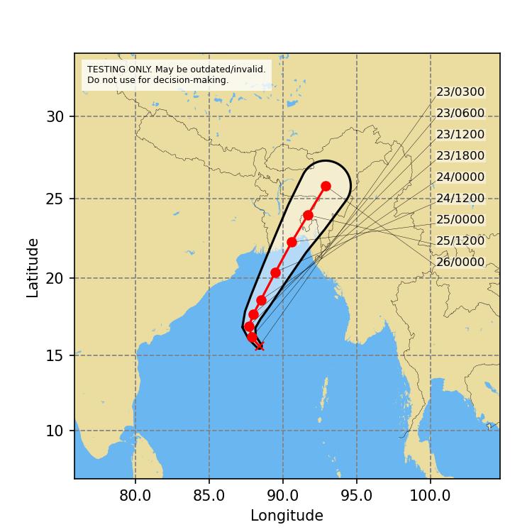
• October 23, 6:30 UTC: RSMC New Delhi issues a storm surge guidance in a Special Tropical Weather Outlook for the North Indian Ocean. The warning predicts a tidal wave of about 2 m height above astronomical tide inundating low lying areas of coastal Bangladesh near the landfall area, and states that astronomical tide of about 5-6 m height (range?) is likely along and off West Bengal - Bangladesh coasts on October 25. Figure 10 shows the track forecast and cone of uncertainty based on the data published in the bulletin (see the bulletin for IMD's authoritative figure).
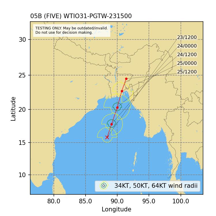
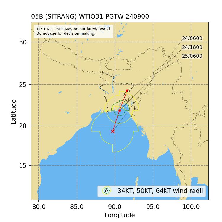
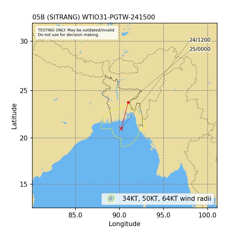
• October 23, 13:59 UTC: The Joint Typhoon Warning Center (JTWC) issues a Tropical Cyclone Formation Alert (WMO GTS header WTIO31 PGTW 231500). Figure 11 shows the track forecast and wind radii published in the bulletin. JTWC forecasts a 34 (50) knots wind radius of 120 (40) nautical miles in both the north-western and north-eastern quadrants valid on October 24 at 12:00 UTC. Later JTWC forecasts are shown in Figure 12 and Figure 13.
• October 23, 18:00 UTC: RSMC New Delhi issues a TC advisory based on 15:00 UTC, in which the storm surge warning is increased to 2.4 m height above astronomical tide.
• October 24, 15:00 UTC: RSMC New Delhi issues a TC advisory based on 12:00 UTC, in which the storm surge warning is decreased to 2 m height above astronomical tide and the likely inundation of low lying areas of coastal Bangladesh near the landfall area is forecast to occur within the next 6 hours and decrease thereafter.
• October 24, 21:00 UTC: In a TC advisory based at 18:00 UTC on October 24, RSMC New Delhi states that Sitrang crossed the Bangladesh coast between 16:00 and 18:00 UTC. The advisory states that a tidal wave of about 1 m height above astronomical tide is likely to inundate low lying areas of the Bangladesh coast during the next 3 hours and gradually decrease thereafter.

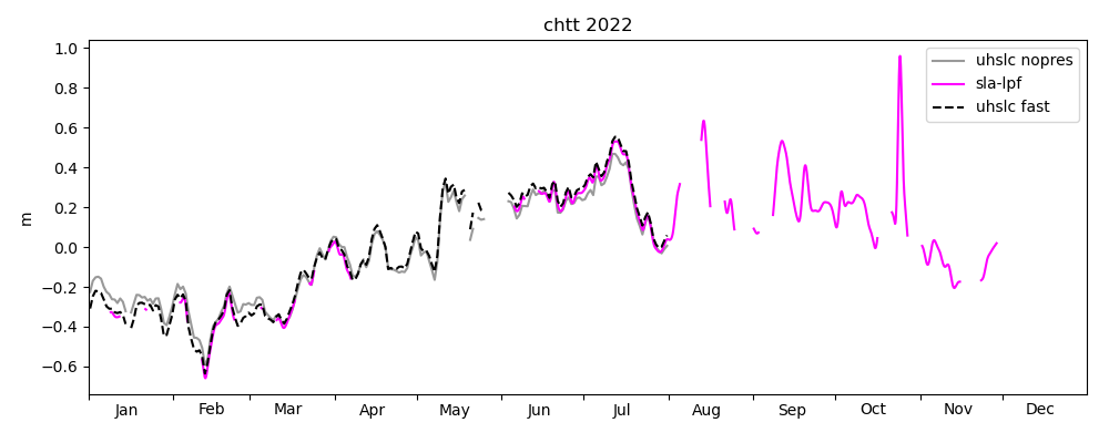
Cyclone Sitrang occured in October 2022, about a month before the writing of this blog post. At the time of writing, no quality-controlled (and also no "fast-delivery") tide gauge data was available in globally accessible tide gauge databases, to our knowledge. To compare model results for cyclone Sitrang, we attempt to create a data processing pipeline from scratch. Comprehensive validation of this method is beyond the scope of this note, but a quick visual assessment can be made by comparing our low-pass filtered sensor data (SLA-LPF) with data from the Joint Archive for Sea Level (JASL, see Caldwell et al. 2015), maintained by the University of Hawaii Sea Level Center (UHSLC) . In addition to their "research quality" data set, UHSLC offers a "fast delivery" (here denoted as UHSLC-FAST) channel with less comprehensive quality control, but more recent data. At the time of writing, the research quality set contained data until 2018 at Chattogram, whereas the fast delivery resource contained data until July 2022. We use the fast delivery data here, keeping in mind the possibly incomplete quality control. Figure 15 shows sea level at Chattogram for the year 2020 from UHSLC-FAST (daily), our SLA-LPF, and UHSLC-FAST with an atmospheric pressure correction applied (henceforth UHSLC-NOPRES). SLA-LPF corresponds well to UHSLC-FAST, but has larger data gaps and is often shifted slightly downward compared to UHSLC-FAST. The data gaps may be caused by a too strict "gap-invalidation" method, i.e. we remove data points separated by more than 10 minutes from the raw data. While this causes gaps in the final time series, it yields sufficient data for harmonic analysis and, importantly in the context of this note, does not yield gaps during the extreme event caused by cyclone Sitrang. Differences in oscillations may be caused by the different number of tidal constituents used to compute the "residual" that is fed into the low-pass filter, and possibly differences in the low-pass filter itself (see section 2). Note also that UHSLC may have used a different instrument than we did. The downward shift may be present because we plot UHSLC-FAST relative to its yearly mean value, whereas SLA-LPF is plotted relative to the mean value computed by the harmonic analysis method. For harmonic analysis, we used sensor data from 2020/01/01 00:00 UTC to 2022/09/07 04:00 UTC, which yielded about 2.6 years of valid hourly data. Note that a comprehensive definition of a mean sea level serving as a tidal datum would presumably involve harmonic analysis over at least a lunar-nodal period (about 18.6 years), and this is beyond the scope of this blog post.

Statistical metrics for the quality of SLA-LPF as compared to UHSLC-FAST can be obtained from overlapping segments of both time series. For the exemplary year 2020, the statistics are:

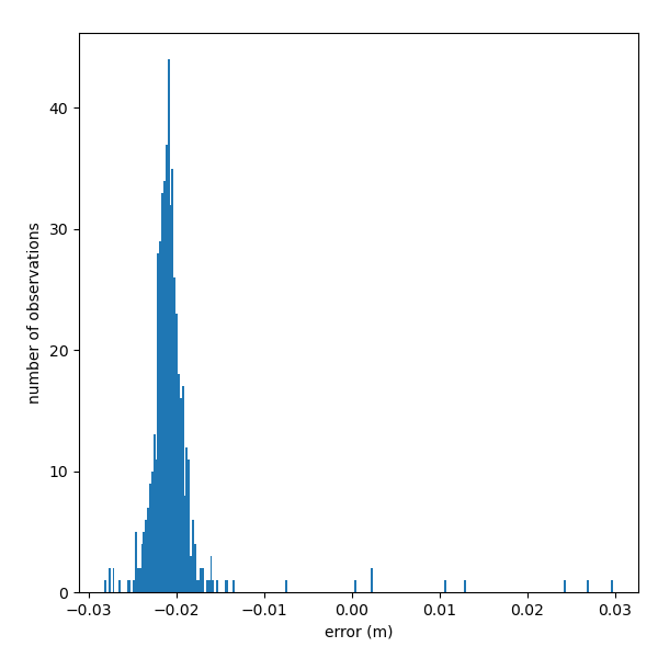
It may be unclear how conclusive these statistics are. Note again that we use the fast-track (non-quality controlled) UHSLC data for comparison. Also, UHSLC distributes its low-pass filtered ("daily") series with a temporal resolution of one day. We assume that it is a subsampled version of an hourly data set, because the low-pass filter is presumably applied to an hourly time series, and digital filters typically do not alter the temporal resolution of a time series (just its spectral composition). For a proper comparison, it may be preferable to compare the filtered time series at their original resolution. Also not that the correlation has been computed by interpreting the patchy input series as one continuous time series, i.e. the end point of a continuous patch followed by a gap, and the starting point of the next continuous patch after the gap are treated as two adjacent data points. The quantitative implications are currently unclear to us. Figure 14 shows a histogram quantifying the differences between between SLA-LPF and UHSCL-FAST for overlapping daily values. The negative bias is related to the definition of the reference level for anomaly computation, which is chosen arbitrarily. The distribution is skewed and the range of differences is roughly 6 cm.

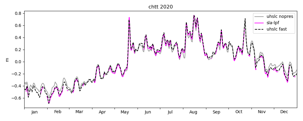
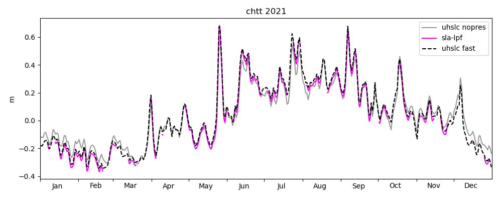
Sea level pressure along the coast of Bangladesh has a climatological high (low) in winter (summer). Since neither NEMO-CMEMS, nor ROMS (in our specific configuration) simulate the effect of atmospheric pressure variations on sea level, the "inverse barometer correction" is applied to observed data before comparing it with model data. For simplicity we use ERA5 sea level pressure for the correction. The result is shown as gray lines in Figures 15-17. The amplitude of the seasonal cycle seems slightly lower for the pressure-corrected time series. Badhan et al. (2016) show climatological seasonal variation of sea level pressure pressure in Chattogram based on data between 1975-2014 (their Fig. 2a). Based on visual inspection of their figure, the seasonal range is roughly 12 hPa, which corresponds to a hydrostatic pressure exerted by a roughly 12 cm high water column.

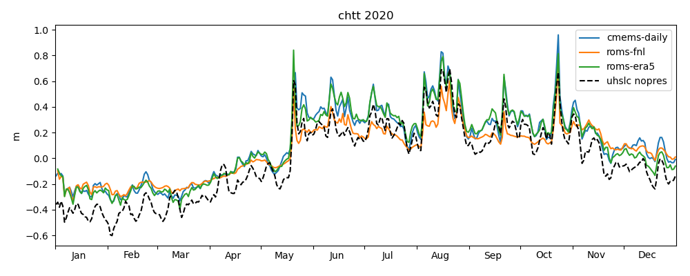
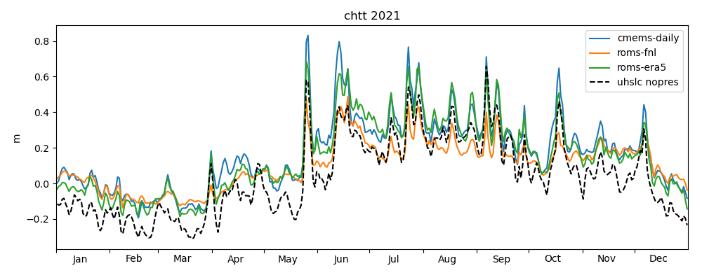
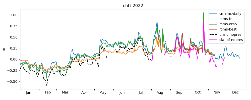
Figures 18-20 show a comparison of modelled sea level anomaly at the Chattogram tide gauge for the years 2020, 2021 and until November 2022 for three models: NEMO-CMEMS, ROMS-FNL and ROMS-ERA5. Observed daily averaged data is shown from UHSLC-FAST with inverse barometer correction applied. The observed data is plotted relative to its yearly mean, whereas model data is plotted relative to the NEMO-CMEMS mean dynamic topography. By "mean dynamic topography" we mean the "mdt" variable distributed in the static datasets of NEMO-CMEMS. As discussed in the previous section, we currently do not understand the relatively large offset of the "mdt" field and the temporal mean of NEMO-CMEMS' free surface over the last couple of years. However, the offset may be of little relevance to the present study. Oscillations on timescales of days-weeks generally agree with observations both in phase and amplitude. All models reproduce the seasonal cycle, i.e. the low (high) sea level anomaly in winter (summer). ROMS-FNL seems to underestimate the amplitude of the seasonal cycle, and oscillations at higher frequencies seem to be of smaller amplitude than compared to NEMO-CMEMS, which may be due to the different atmospheric forcing. Consistent with this hypothesis is that ROMS-ERA5, which is forced with an ECMWF product (like NEMO-CMEMS, although with a reanalysis and presumably with different flux parameterizations), seems visually more similar to NEMO-CMEMS. Similar interpretations hold for the years 2021 and 2022. Figure 20 shows the ROMS-BEST series for the interval in which we deployed the "operational" toy model, covering the occurence of TC Sitrang. ROMS-BEST is a patched sequence of multiple experiments. For each model simulation, the second day is extracted and appended to the sequence (loosely following Wilkin et al. 2019, but note again that no assimilation is performed in the toy model). Comparing ROMS-BEST with ROMS-FNL, the former seems to have a variance much closer to observations. We are unaware of any reasons why an experiment forced with GFS (ROMS-BEST) should have consistently lower variance than an experiment forced with GDAS/FNL (ROMS-FNL). This raises the suspicion that the poor performance of ROMS-FNL is due to a processing error on our part. Another possibility may be a steadily deteriorating representation of circulation and water masses in the multi-year experiment, but the ROMS-FNL variance seems to be consistently low even in the first months of the experiment.

Figures 21-23 show Taylor diagrams for the sea level produced by the long-period model simulations at the Chattogram tide gauge. Taylor (2001) proposed diagrams for assessment of pattern similarity based on statistical quantities. The general idea is to visualize four related key statistical quantities, i.e. the centered pattern RMS difference \(E^{\prime}\) between two variables \(f\) and \(r\), their standard deviations \(\sigma _{f}\) and \(\sigma _{r}\), and their correlation coefficient \(R\). These are related by

The term centered (using the terminology of Taylor, 2001) refers to the prior removal of a possibly existing mean, which in the present case is the reference level for the definition of sea level anomaly and not further discussed. The reference data for the diagram in Figure 21 is UHSLC-NOPRES, since model performance in the current configuration should be evaluated against a time series with inverse barometer correction. ROMS-FNL has the lowest standard deviation, consistent with the seemingly too low oscillations in the time series plots above. NEMO-CMEMS apparently not only has a more accurate standard deviation, but is also slightly better correlated with the observation. ROMS-ERA5 performs almost identically to NEMO-CMEMS on the Taylor diagram. Finally, the observation UHSLC-FAST is also shown for comparison. The structure of the Taylor diagrams for 2021 and 2022 are broadly similar to the one of 2020.

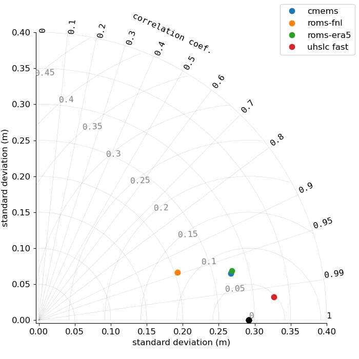
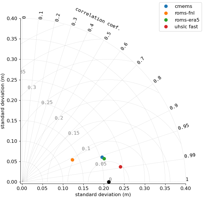
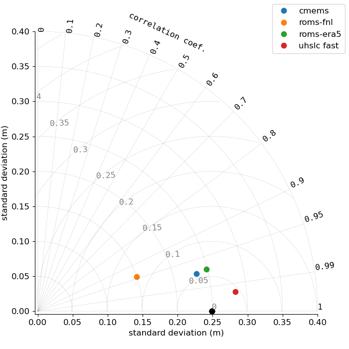
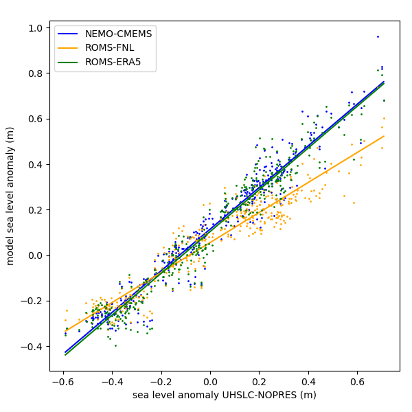
Figure 24 shows a scatter plot comparing observed and modelled water levels. The slopes of the linear least-square fits are 0.92 (NEMO-CMEMS), 0.66 (ROMS-FNL) and 0.92 (ROMS-ERA5).

Figure 25 shows water level at the Chattogram tide gauge in a 5-day window containing the extreme event caused by cyclone Sitrang. The shown sensor data was cleaned of spikes (if any) and the tidal prediction from the harmonic analysis step was subtracted. The tidal prediction contains only diurnal or higher frequencies. No atmospheric pressure correction was applied, and the pressure correction is shown as a separate line. The semi-diurnal oscillations of the sensor residual before and after the extreme event with amplitudes of about 0.25 m are typical for tidal residuals at the Chattogram tide gauge (see e.g. our previous blog post). We do not know whether they result from inaccuracies of our harmonic analysis or are merely transiently periodic responses to internal variability or possibly non-periodic meteorological forcing. Given these uncertainties, one could crudely estimate the storm-induced sea level rise to be about 2 m. This agrees with the prediction in the advisories of RSMC New Delhi extracted above. We have no data regarding possible influences of water level rise in the Karnaphuli River or the mouths of the GBM basin due to runoff from precipitation. Our toy model is unable to simulate such compound effects, because the Karnaphuli river is not modelled at all, and the GBM discharge is climatological. Figure 25 shows that the SLA-LPF data, which represents averages on daily time scales, severely underestimates the instantaneous peak water level. For comparison, NEMO-CMEMS sea surface anomaly is plotted, both the hourly product and its daily average. Apparently, the interval during the extreme event is flagged as invalid by the NEMO-CMEMS distributors, perhaps to prevent misuse of NEMO-CMEMS data for coastal-scale disaster management.

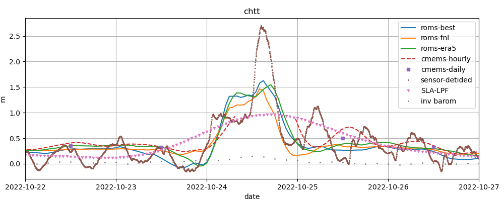
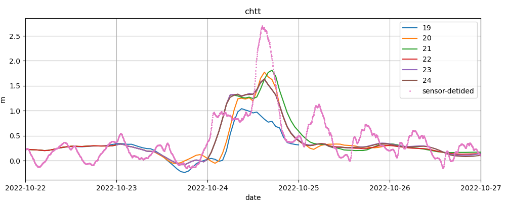
Figure 26 shows all ROMS "forecast" simulations containing data for October 24, 2022. One simulation is performed each day (D0), and each simulation covers 6 days from D-3 to D+2. The first simulation is performed on October 22 and covers the interval from October 19 at 00:00 UTC to October 24 at 24:00 UTC. The second run is performed on October 23 and covers October 20 to 25, etc. According to the NEMO-CMEMS documentation (see section 3), assimilation runs for days D-14 to D-1 are performed each week on Wednesdays. Consider our run performed on October 27 covering the 6 day window starting from October 24. October 27 is a Thursday, hence this run may have benefited from CMEMS-NEMO assimilation performed on Wednesday, October 26 (if we understand the CMEMS-NEMO schedule correctly). In some experiments, we noted spurious oscillations of sea level that dissipated after a couple of days. We speculate that they result from the sudden, weekly change in boundary conditions reflecting the increments of the NEMO-CMEMS analysis, but this has not been further investigated. One way to mitigate this problem may be to extend the 6-day windows (D-3 to D+2) to windows starting at D-14 once per week, in synchronization with the NEMO-CMEMS schedule.

References

- Amante, C., Eakins, B.W., 2009: ETOPO1 1 Arc-Minute Global Relief Model: Procedures, Data Sources and Analysis. NOAA Technical Memorandum NESDIS NGDC-24.
- Badhan, M.A., Farukh, M.A., Baten, M.A., Hossen, M.A.M., Biswas, S., Parvej, M.S., 2016: Sea level pressure variation and major cyclone events in coastal regions of Bangladesh.
- Blackadar, A.K., Tennekes, H., 1968: Asymptotic similarity in neutral barotropic planetary boundary layers.
- Blayo, E., Debreu, L., 2005: Revisiting open boundary conditions from the point of view of characteristic variables.
- Bourdallé-Badie, R., Treguier, A.M., 2006: A climatology of runoff for the global ocean-ice model ORCA025.
- Caldwell, P.C., Merrifield, M.A., Thompson, P.R., 2015: Sea level measured by tide gauges from global oceans — the Joint Archive for Sea Level holdings (NCEI Accession 0019568), Version 5.5, NOAA National Centers for Environmental Information, Dataset, doi:10.7289/V5V40S7W.
- Caldwell, P.C., 2015: Hourly Sea Level Data Processing and Quality Control Software: Version for Linux Operating Systems. SLP64 User Manual
- Codiga, D.L., 2011: Unified tidal analysis and prediction using the UTide Matlab functions. Technical Report 2011-01.
- Dai, A., Trenberth, K.E., 2002: Estimates of freshwater discharge from continents: Latitudinal and seasonal variations.
- Dutour-Sikirić, M., Janeković, I., Kuzmić, M., 2009: A new approach to bathymetry smoothing in sigma-coordinate ocean models.
- Fairall, C.W., Bradley, E.F., Rogers, D.P., Edson, J.B., Young, G.S., 1996: Bulk parameterization of air‐sea fluxes for tropical ocean‐global atmosphere coupled‐ocean atmosphere response experiment.
- Federal Institute of Hydrology (BfG), Germany, 2020: Basins and Sub-Basins / Global Runoff Data Centre, GRDC.
- Fekete, B.M., Vörösmarty, C.J., Grabs, W., 2002: High‐resolution fields of global runoff combining observed river discharge and simulated water balances.
- Flanders Marine Institute (VLIZ), Intergovernmental Oceanographic Commission (IOC), 2022: Sea level station monitoring facility.
- Flather, R.A., Davies A.M., 1975: The application of numerical models to storm surge prediction.
- Flather, R.A., 1976: A tidal model of the northwest European continental shelf.
- Flather, R.A., 1987: A tidal model of the northeast Pacific.
- GEBCO Compilation Group, 2008: The GEBCO_08 Grid, version 20100927
- GEBCO Compilation Group, 2021: GEBCO 2021 Grid (doi:10.5285/c6612cbe-50b3-0cff-e053-6c86abc09f8f)
- Grant, W.D., Madsen, O.S., 1986: The continental-shelf bottom boundary layer.
- Harris, C.R., Millman, K.J., van der Walt, S.J., others, 2020: Array programming with NumPy.
- Hedstrom, K., Torgerson, B., Hadfield, M., Dussin, R., Pringle, J., Dunphy, M., Wang, C., 2020: ESMG/pyroms: v1.0 for use with Python3 (v1.0.0).
- Hersbach, H., Bell, B., Berrisford, P., Hirahara, S., Horányi, A., Muñoz‐Sabater, J., others, 2020: The ERA5 global reanalysis.
- Hunter, J.D., 2007: Matplotlib: A 2D Graphics Environment.
- India Meteorological Department, 2021: CYCLONE WARNING IN INDIA STANDARD OPERATION PROCEDURE
- Jana, S., Gangopadhyay, A., Chakraborty, A., 2015: Impact of seasonal river input on the Bay of Bengal simulation.
- Lehner, B., Grill G., 2013: Global river hydrography and network routing: baseline data and new approaches to study the world’s large river systems.
- Lellouche, J.M., Greiner, E., Bourdallé-Badie, R., Gilles, G., Angélique, M., Drévillon, M., et al., 2021: The Copernicus global 1/12 oceanic and sea ice GLORYS12 reanalysis.
- Lellouche, J.M., Greiner, E., Le Galloudec, O., Garric, G., Regnier, C., Drevillon, M. et al., 2018: Recent updates to the Copernicus Marine Service global ocean monitoring and forecasting real-time 1/12 high-resolution system.
- López, A.G., Wilkin, J.L., Levin, J.C., 2020: Doppio-a ROMS (v3.6)-based circulation model for the Mid-Atlantic Bight and Gulf of Maine: configuration and comparison to integrated coastal observing network observations.
- Marchesiello, P., McWilliams, J.C., Shchepetkin, A., 2001: Open boundary conditions for long-term integration of regional oceanic models.
- Martinho, A.S., Batteen, M.L., 2006: On reducing the slope parameter in terrain following numerical ocean models.
- National Centers for Environmental Prediction/National Weather Service/NOAA/U.S. Department of Commerce., 2015: NCEP GDAS/FNL 0.25 Degree Global Tropospheric Analyses and Forecast Grids (updated daily). Research Data Archive at the National Center for Atmospheric Research, Computational and Information Systems Laboratory. Accessed 16 November 2022
- Pugh, D.T., 1987: Tides, surges and mean sea-level: a handbook for engineers and scientists.
- Reid, R.O., Bodine, B.R., 1968: Numerical model for storm surges in Galveston Bay.
- Shchepetkin, A.F., McWilliams, J.C., 2005: The regional oceanic modeling system (ROMS): a split-explicit, free-surface, topography-following-coordinate oceanic model
- Southard, J., 2019: Introduction to Fluid Motions and Sediment Transport.
- Taylor, K.E., 2001: Summarizing multiple aspects of model performance in a single diagram.
- U.S. Integrated Ocean Observing System, 2021: Manual for Real-Time Quality Control of Water Level Data Version 2.1: A Guide to Quality Control and Quality Assurance of Water Level Observations.
- UNESCO/IOC, 2020: Quality Control of in situ Sea Level Observations: A Review and Progress towards Automated Quality Control, Vol. 1.
- Wilkin, J., Arango, H., Hunter, E., Levin, J., Lopez, A., Moore, A., Zavala-Garay, J., 2019: The MARACOOS ROMS 4D-Var "Doppio" Operational Data Assimilative Ocean Forecast System for Northeast U.S. Coastal Waters