Correction (v1) to "A simplistic operational toy model of the northern Bay of Bengal"
Riha, S.1 Abstract
We correct erroneous results shown in a previous blog post, which were induced by incorrectly imposing radiative fluxes in an experiment forced with GDAS/FNL atmospheric fields. In the previous blog post, we used sea level variation measured at a single tide gauge as a metric for preliminary model validation. The poor model performance found previously when using GDAS/FNL was induced by a severe deterioration of water mass representation in the model, which apparently also affected the sea level variation. Here we present results of the multi-year simulations with improved application of radiative fluxes. Based on the single metric used previously, the ROMS solution forced with GDAS/FNL now performs about as well as the one forced with ERA5. Corrections and comments via E-mail are appreciated.
2 Introduction
In a previous blog post we described two multi-year simulations that differed only in atmospheric forcing. For the first experiment, we used NCEP FNL (Final) operational global analysis and forecast data from the Global Data Assimilation System (GDAS) (NCEP, 2015). The second simulation was forced with the ERA5 global reanalysis (Hersbach et al., 2020). Comprehensive validation of circulation and water mass properties is pending, and we reported on a preliminary validation using only one single instrument. The instrument is a tide gauge located in Chattogram, Bangladesh, adjacent to a wide and shallow shelf and in relative proximity to the Ganges-Brahmaputra-Meghna delta. Based on the single metric, model performance using GDAS/FNL was significantly worse than using ERA5. Modelled sea level at the tide gauge had lower correlation and much lower variance relative to the observed time series. On the other hand, a short simulation using a "toy-operational" version of the model forced with GFS, did not show the lack of variance visible in the long-term simulation. The fact that GDAS/FNL and GFS are produced by a similar numerical model, raised the suspicion that the poor performance of GDAS/FNL was due to a processing error made by the author. Indeed, inspection of the water mass properties of the GDAS/FNL simulation showed that the surface temperature field degraded at a rate that produced minimum surface temperatures of about 5 degrees C in the Bay of Bengal during the first 6 simulated weeks (not shown), which corroborated the suspicion of a processing error in the atmospheric forcing. We found that radiation fluxes, which are retrieved from GDAS/FNL and serve as input to the bulk flux parametrization of Fairall et al. (1996), were erroneously held constant during the simulation. During the fix of this error, another error was encountered which lead to an incorrect interpretation of 3-hour averaged radiation fluxes as 6-hour averaged radiation fluxes.
In the following section we present the corrected version of the figures shown initially in the previous blog post.
3 Results
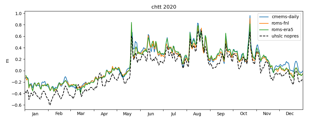
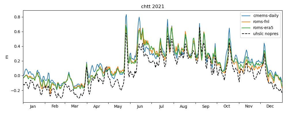
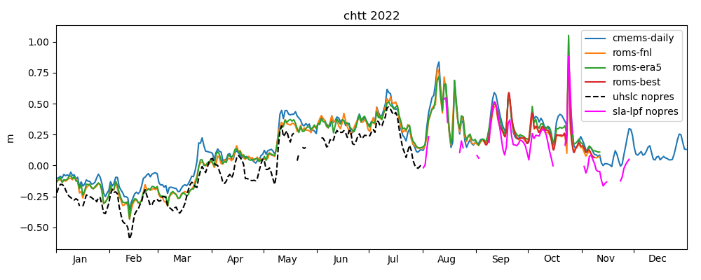
Figures 18-20 of the previous post showed a comparison of the modelled sea level anomaly and observed, daily averaged data. The corrected versions are shown in Figures 1-3. Apart from the correction of the radiative fluxes described above, a further correction was applied to the computation of the inverse barometer effect. In the previous blog post, we forgot to apply the daily filter on the atmospheric pressure field used to compute the inverse barometer effect. Since this field has a temporal resolution of 3 hours, we speculate that it may resolve atmospheric tides in the diurnal band and above, and should probably be removed. We have not quantified the effect of the filter, but based on visual inspection of Figures 1-3, the effect does not seem to be large compared to the previous version of the figures. Hence, this issue is not further discussed here.
ROMS-FNL simulates the seasonal cycle much better than previously, and the oscillations at higher frequencies now seem to have similar amplitude as the other models.
Figures 4-6 show the corrected Taylor diagrams, confirming the now improved performance of ROMS-FNL.
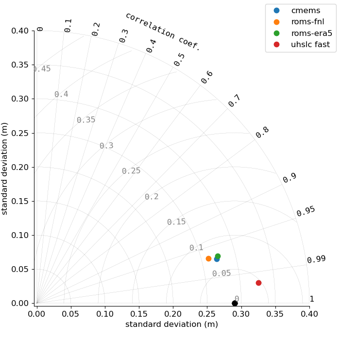
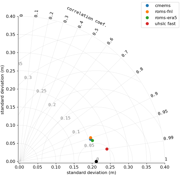
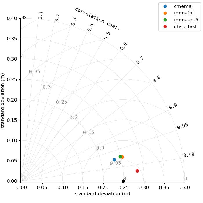
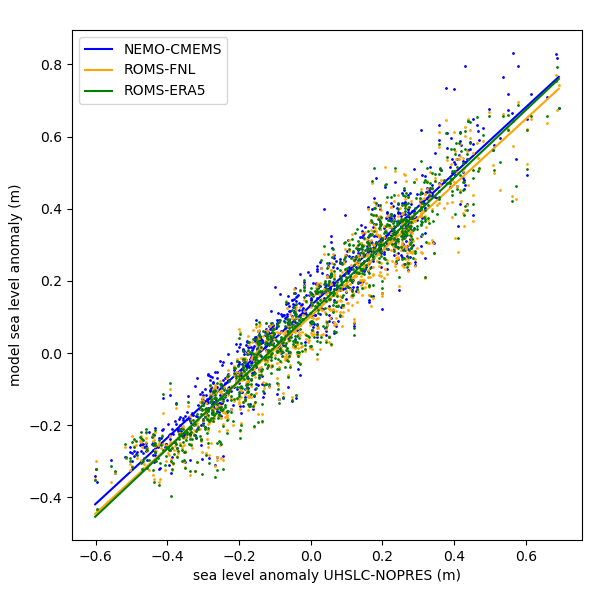
Figure 7 shows the corrected scatter plot comparing observed and modelled water levels. Note that in this context, yet another "error" was found in the previously used processing scripts. Previously, the scatter plot showed only data from 2020, although we intended to show the period from 2020 to July of 2022. This is corrected now and the slopes of the linear least-square fits are 0.92 (NEMO-CMEMS), 0.91 (ROMS-FNL) and 0.94 (ROMS-ERA5). The numbers for NEMO-CMEMS and ROMS-ERA5 are similar to the ones published previously, but the slope of ROMS-FNL is now much closer to 1.
4 Summary and discussion
We present corrected results of a previous blog post, where we used numerical ocean models of the northern Bay of Bengal to simulate water level variations at the location of a tide gauge. In the previous post we based a preliminary model validation on this single metric, and found poor performance when using GDAS/FNL fields for atmospheric forcing. Since the publication of the previous post, we found that we had incorrectly applied GDAS/FNL radiative fluxes, which lead to a severe deterioration of water mass representation in the model, and apparently also affected the sea level. Here we presented results of the multi-year simulations with improved application of radiative fluxes. The ROMS solution forced with GDAS/FNL now performs about equally as the one forced with ERA5.
Although the incorrect application of radiation fluxes affects the sea level variation at the tide gauge, the effect on the surface temperature field is more severe. The error would have been caught earlier, if the previous simulations were to have been accompanied by a more comprehensive validation including water mass properties. In this case, the error would have been caught even using GDAS/FNL as the only forcing type. Using instead only the sea-level metric, the suspicion of an error was raised somewhat indirectly, by comparing multiple atmospheric forcings, and consequently their custom-tailored preprocessing methods.
Regarding the use of radiation fluxes from GDAS/FNL and GFS, we are still unsure if we apply them in the optimal way. The maintainers of the GDAS/FNL and GFS data sets seem to publish radiation fluxes which represent averages between synoptic times (hours 0, 6, 12 and 18) and "valid times", i.e. the times for which a forecast is published. For the results shown above, we impose radiation fluxes with 6-hourly resolution, even though one could (if we understand correctly) compute average radiation fluxes at a 3-hourly resolution from the available data. In hindsight, this note should have included a comparison with 3-hourly radiation fluxes. ROMS-FNL might then perform even better. This is deferred to future work.
References
- Fairall, C.W., Bradley, E.F., Rogers, D.P., Edson, J.B., Young, G.S., 1996: Bulk parameterization of air‐sea fluxes for tropical ocean‐global atmosphere coupled‐ocean atmosphere response experiment.
- Hersbach, H., Bell, B., Berrisford, P., Hirahara, S., Horányi, A., Muñoz‐Sabater, J., others, 2020: The ERA5 global reanalysis.
- National Centers for Environmental Prediction/National Weather Service/NOAA/U.S. Department of Commerce., 2015: NCEP GDAS/FNL 0.25 Degree Global Tropospheric Analyses and Forecast Grids (updated daily). Research Data Archive at the National Center for Atmospheric Research, Computational and Information Systems Laboratory. Accessed 16 November 2022
