2 Introduction

Storm surges are increases of sea level in coastal areas, caused by severe wind. They typically occur on time scales ranging from hours to several days, and the associated inundation can cause massive destruction in densely populated areas. Risk assessment studies aim to estimate the likelihood of rebuilding costs corresponding to the probability that a storm surge event exceeds a certain intensity. To this end, vulnerability functions are constructed, which relate flood inundation depth with the cost of repair of a particular asset (e.g. USACE 2015). The mapping between sea water inundation probabilities and storm event probabilities is achieved by feeding a representative set of storms into a numerical storm surge model, which deterministically translates the storm to inundation depths. To obtain robust statistics, a large number of model simulations may be performed (but see e.g. Taflanidis et al. 2013). For example, NOAA's SLOSH model (Jelesnianski et al., 1992) has been used by Lin et al. (2010) in a model-based storm surge risk assessment study for New York City. SLOSH is a low-complexity model that allows hundreds or thousands of simulations in the course of an assessment study.

In this post we outline the components of a minimal numerical model to obtain storm surge water heights along a curved coast with variable bathymetry. We discretize the simplest possible mathematical model that can be expected to yield useful results. The simulated surges may be used as boundary conditions for simple inundation models covering terrain, e.g. static "bathtub" models or possibly more complex hydraulic models covering terrain only, or shallow parts of the continental shelf. The simplicity of the model may limit it to qualitative assessment studies, and perhaps makes it useful for educational purposes.

We empirically justify the mathematical model a posteriori without prior scaling analysis. We do this simply by simulating the hurricane Sandy event in 2012, followed by a comparison to observations. Forcing fields are obtained from the parameterized wind model used in the SLOSH model, with parameters obtained from a hindcast simulations.

3 Model components

We solve the equations

U_{, t} = - g (D + h) (h - h_{0})_{, x} + τ_{x}

V_{, t} = - g (D + h) (h - h_{0})_{, y} + τ_{y}

h_{, t} = - U_{, x} - V_{, y}

where

$U, V$	components of transport
$- g$	downward gravitational acceleration
$D$	depth of unperturbed water
$h$	height of water surface relative to a chosen datum
$h_{0}$	height of water surface due to atmospheric pressure variations
$τ_{x}, τ_{y}$	components of surface stress

$D$ , $h$ and $h_{0}$ are measured relative to a common chosen datum, and the subscripts preceeded by commas denote partial derivatives. The mathematical notation follows Jelesnianski et al. (1992). Our choices for spatial discretization, lateral boundary conditions and surface forcing also follow Jelesnianski et al. (1992) and are further detailed below. However, our mathematical model is significantly less sophisticated and complete than SLOSH's, due to 1) the general lack of the coriolis terms, and 2) the parameterization for the effects of bottom friction. Note the lack of any dissipation mechanism in the analytical model.

4 Forcing

We use the SLOSH parametric wind model ( Jelesnianski et al. 1992; Jelesnianski and Taylor 1973) to obtain the wind stress vectors, given by

τ = C_{D} \frac{ρ_{a}}{ρ_{w}} | W | W

where $C_{D}$ is the drag coefficient, $ρ_{a}$ and $ρ_{w}$ are densities of air and water, and $W$ is the surface wind velocity. Following Jelesnianski et al. 1992, we use a value of $3 \cdot 10^{- 6}$ for $C_{D} ρ_{a} / ρ_{w}$ . The wind velocity $W$ is composed of

W = V + V_{1}

where $V$ is the velocity of a stationary storm, and $V_{1}$ is an empirical vector correction for storm motion. As input parameters to the parametric wind model, we use 6-hourly data from the Tropical Cyclone Extended Best Track Dataset (EBTR) (Demuth et al., 2006). The following parameters are used:

Track position
Minimum central pressure $p_{m i n}$
Radius of maximum wind speed $R$
Pressure of the outer closed isobar $p_{a m b}$
Radius of the outer closed isobar

First we define a target pressure difference $Δ p$ as

Δ p = p_{a m b} - p_{m i n}

and choose a wind speed profile

V (r) = V_{R} \frac{2 R r}{R^{2} + r^{2}},

where $r$ is a radial coordinate and $V_{R}$ is an arbitrary speed. Following Jelesnianski and Taylor (1973), we integrate the velocity profile to obtain the corresponding pressure distribution for a stationary storm. We describe the integration method of Jelesnianski and Taylor (1973) in a separate post. In an iterative procedure, we then adjust the arbitrary $V_{R}$ until the pressure distribution yields $Δ p$ up to a small error.

We take the most basic approach and run the parametric wind model only for each 6-hourly parameter set. We do not interpolate the parameters to intervals smaller than 6 hours. For the simulated interval from 00:00 hours on October 28, 2012, to 06:00 hours on October 31, this yields 14 fields of $h_{0}$ and $τ$ . For the model integration, we linearly interpolate between these 14 snapshots. This approach is arguably crude, and the degree of realism of the resulting fields will not be assessed here.

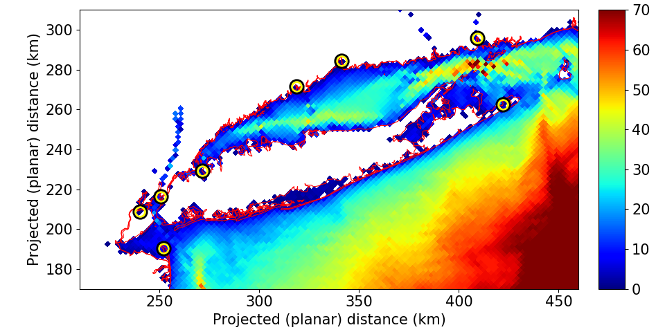
Figure 1 shows the wind speed field in miles per hour, roughly 6 hours before landfall. We choose imperial units for this plot, to facilitate comparison with figure 20 of Forbes et al. (2014), who assessed SLOSH's performance for hurricane Sandy. Segments of the blue line connect discrete 6-hourly hindcast track positions, for each of which parameters were extracted from EBTR data. Missing values for radius of maximum wind and ambient pressure after October 30, 12:00, are substituted with the most recent available values. Although this is a crude approximation, it is made 12 hours after landfall, and hence is unlikely to affect the peak surge. The cyclone propagation direction for computation of the asymmetry in the wind speed field is defined for simplicity as the direction of the linear segment connecting the current track position to the next one. For the case shown in figure 1, the direction for October 29, 18:00, is taken to be the direction of the segment leading to the landfall location.

Snapshot of wind forcing before landfall. — Figure 1: **Color shading** shows wind speed in miles per hour, roughly 6 hours before landfall. Only values within the model domain are shown. The **blue segments** connect 6-hourly hindcast track positions of hurricane Sandy, with **black labels** indicating time in UT. **White arrows** show wind direction and magnitude in convenient units. The coastline is shown in **black**.

Figure 2 shows the wind speed at landfall, and it is interesting to discuss the differences to figure 20 (top panel) of Forbes et al. (2014), which shows their wind field for the same time. First, note that our inflow angles are apparently smaller than those of Forbes et al. (2014). Second, the asymmetry of our wind field seems to be rotated slightly in counter-clockwise direction relative to Forbes et al. (2014). Third, our maximum wind speed seems to be lower by roughly 5-10 miles per hour. The first and second properties are consistent with each other in the context of SLOSH's parametric wind model. In this model, the maximum wind speed always occurs in the right rear quadrant of the storm, and larger inflow angles can cause the maximum to shift more towards the rear, where the stationary storm velocity is exactly parallel to the propagation direction of the storm. The cause for the differences to Forbes et al. (2014) remain unclear to us. It should be noted that the fields of Forbes et al. (2014) seem to be quantitatively more similar to a reanalysis wind field, which is depicted in the lower panel of their figure 20.

Snapshot of wind forcing at landfall. — Figure 2: As Figure 1, but for the approximate time of landfall.

5 Bathymetry and topography

Bathymetric and topographic data are extracted from the ETOPO1 global relief model with 1 arc-minute resolution (Amante et al., 2009), which corresponds to about $1852 m$ ( $1404 m$ ) in northward (eastward) direction around New York City. The authors of the data set refer to the vertical datum simply as "sea level", indicating that the various specific vertical datums (mean sea level, mean high water, mean low water) differ by less than the vertical accuracy of ETOPO1, which is specified as "10 meters at best". The low vertical accuracy further implies that the topography data is not well suited for inundation studies (especially in comparison to other data sets available for the area of interest), which further motivates the lack of inundation processes in our model. Note, however, that the use of lateral wall-boundary conditions is generally be problematic. They may increase surge levels along the wall, where in reality, any accumulated water would constantly propagate landwards.

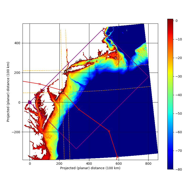
We project the extracted ETOPO1 data onto a rectangular and equidistant grid, using an oblique Mercator projection. We accept any distortions of area and cardinal directions relative to the grid lines. Figure 3 shows a visualization of the angle distortions, in which sample meridians and parallels are drawn as dashed orange lines. Consider, for example, the grid boundary running in north-eastward direction from the origin of the projection plane. This line has an azimuth of roughly 45 degrees at the origin, but at New York City, the azimuth is slightly larger. In the computation of our surface forcing, we ignore this distortion. For example, we compute wind stress vectors via the SLOSH parametric wind model in the projection plane, and the distortion implies that if two vectors at different locations point in the same direction in the projection plane, they do not have the same azimuth in reality. The angle distortions are even more obvious looking at the curved parallels. It is essential to note, however, that the projection chosen in this study is not the optimal oblique Mercator projection for the domain under consideration. The origin of the projection plane, and hence the minimal angle distortions, could easily be moved into the center of the domain. This is deferred to a later article. All projections have been computed with the open source proj and geod programs ( Evenden 1990; Evenden 2005). A more detailed description of the oblique Mercator projection can be found in one of our previous posts

Numerical grid boundaries in the oblique Mercator projection plane. — Figure 3: **Color shading** shows ETOPO1 elevation data in meters below zero. All elevations below $80 m$ are mapped to the darkest color. The **purple** rectangle delineates the grid boundaries, the **red** line shows the hindcast track of hurricane Sandy, **black circles** indicate the location of NOAA's tide gauge stations. The projection is an oblique Mercator projection whose projection cylinder is oriented such that the line of true scale runs along the purple line that is mostly on land, i.e. the line emanating from the origin of the projection plane with an azimuth of about 45 degrees. To visualize the distortion of the cardinal directions on the projected grid, sample meridians and parallels are shown as **dashed orange**. Note, for example, that the angle between the purple line and the meridian intersecting with New York City is slightly *larger* than 45 degrees.

In line with the minimal ETOPO1 resolution of one nautical mile, we choose roughly one nautical mile as the grid spacing for our equidistant grid. Due to the area distortion of our projection, the inversely projected area of each grid cell varies slightly, the maximum difference between any two grid cells being about half of a percent. The model bathymetry is shown in figure 4. Grid points drawn in white indicate land, which is initially defined as grid points which are elevated higher than level zero. In a second step, we unmask some land grid points which cover up tide gauges location. In a final step, we set a global minimum depth of $1 m$ for wet grid points. It can be seen in figure 4 that we keep manual manipulation of the land mask to a minimum. No attempt is made to visually align the land mask to the projection of the coastline, except where necessary for validation purposes. Note that one notable feature of the resulting bathymetry is that the East River is closed.

Bathymetry and land mask. — Figure 4: **Color shading** shows depth in meters at wet model grid points, dry points are painted **white**. The **red** line shows the projection of the actual coast line. **Yellow and black** circles indicate locations of tide gauge stations.

6 Discretization

Our choice for spatial discretization, lateral boundary conditions and smoothing for $h$ follows Jelesnianski et al. (1992). For example, we use an Arakawa-B grid, and the scheme for the pressure gradient operator is identical to that given by Jelesnianski et al. (1992) for Cartesian coordinates. Some of the differences to SLOSH are as follows:

The lateral land-sea boundary formed by outcropping topography is treated as a vertical wall with a no-normal-flow boundary condition.
At open boundaries with depths shallower than $22.86 m$ we use the boundary condition suggested by Jelesnianski et al. (1992) for intermediate depth. The implementation of the shallow boundary condition described by Jelesnianski et al. (1992) is currently unclear to us.
We use a simple forward Euler scheme for time integration.
Our mathematical model domain is the projection plane, and the numerical domain is an equidistant grid within the projection plane. A qualitative description of the implied distortions was given above.

Point 1 is an essential functional limitation compared to SLOSH, which is capable of simulating the spreading of water over terrain. This class of flow regimes requires specialized numerical techniques to move boundary conditions and simulate nonlinear flow governed by hydraulic principles. Regarding our validation experiment, neglecting the simulation of inundation is consistent with the vertical accuracy of our model bathymetry and topography (see below).

Note that SLOSH uses a grid of varying resolution whereas we use an equidistant grid. It could be argued that our model is unnecessarily inefficient, since the time step is necessarily bounded by the deepest regions of the domain, which are located along the seaward grid boundary and are about $4500 m$ deep.

7 Validation results

We compare our model results with tide gauge measurements at 13 locations within the model domain (see Figure 3). The data is obtained from the Tides and Currents data portal maintained by the Center for Operational Oceanographic Products and Services. We use time series of the predicted water level (including tides) and the observed water level in 6 minute intervals. Both measurements are referenced to the local mean sea level for the purpose of this study.

Location of NOAA tide gauge stations. — Figure 5: **Blue** markers show locations of NOAA tide gauge stations. The **red** line outlines the hurricane track.

Figure 6 shows a comparison between simulated and observed surge heights, where we define surge as the difference between observed and predicted water levels including tidal variations. The root mean square error ranges from $0.23 m$ at Chatham to $0.62 m$ at Cape May, and the average across stations is $0.37 m$ . The correlations range between $- 0.04$ at Cape May and $0.96$ at Montauk, and the average across stations is $0.79$ . All root mean square errors are larger than those reported by Forbes et al. (2014), and some are more than twice as large (The Battery and Cape May). We note that the computation of the root mean square error is presumably sensitive to the model initialization. The surface height in the domain is set to a constant at the start of the spin-up phase, and the constant is set the mean of the observed surge heights on October 28, 00:00, which is roughly $0.3 m$ . We note that while this procedure may be justifiable in a forecasting context, it is somewhat dubious in a catastrophe modeling context. In the latter, the initial surge should be reproduced by the model as a response to the forcing. A possibly related feature of the present simulation is the relatively consistent underestimation of the surge leading up to to the maximum surge. An attribution of these shortcomings is deferred to a later study.

Comparison between model data and observed data. — Figure 6: **Blue** lines show simulated water height in meters as function of time at various tide gauge stations. The **red** line shows the surge height. $R M S E$ and $C O R R$ denote the root mean square error and correlation. The brackets contain the corresponding values listed by Forbes et al. (2014) in their figure 11.

8 Summary and discussion

We described a minimal, two-dimensional storm surge model with varying bottom topography and parameterized wind forcing. We validated the model by comparing simulation results to observational data from the hurricane Sandy event. The mathematical model is discretized following (Jelesnianski et al., 1992), but is significantly simpler than SLOSH, in that it neither contains a coriolis term, nor a bottom friction parameterization. The model domain is a projection plane, and closed lateral boundary conditions are implemented as vertical walls. The wind forcing is identical to that described by Jelesnianski et al. (1992) and Jelesnianski and Taylor (1973). The model shows some skill in predicting surge heights, with an average root mean square error of $0.36 m$ and a mean correlation of $0.75$ . These statistics are likely sensitive to the initialization of sea level. The currently used initialization procedure is motivated by forecasting applications, and may be inappropriate in the context of catastrophe modeling.

9 Acknowledgements

We thank a member of the Co-ops User Services Team, who explained the significance of the data columns in their API response.

References

Amante, C., Eakins, B.W., 2009: ETOPO1 1 Arc-Minute Global Relief Model: Procedures, Data Sources and Analysis. NOAA Technical Memorandum NESDIS NGDC-24.
Demuth, J., DeMaria, M., Knaff, J.A., 2006: Improvement of advanced microwave sounder unit tropical cyclone intensity and size estimation algorithms.
Evenden, G.I., 1990: Cartographic projection procedures for the UNIX environment: A user's manual
Evenden, G.I., 2005: libproj4: A comprehensive library of cartographic projection functions (preliminary draft)
Forbes, C., Rhome, J., Mattocks, C., Taylor, A., 2014: Predicting the storm surge threat of Hurricane Sandy with the National Weather Service SLOSH model
Jelesnianski, C.P., Chen, J., Shaffer, W.A., 1992: SLOSH: Sea, lake, and overland surges from hurricanes
Jelesnianski, C.P., Taylor, A.D., 1973: A preliminary view of storm surges before and after storm modifications
Lin, N., Emanuel, K.A., Smith, J.A., Vanmarcke, E., 2010: Risk assessment of hurricane storm surge for New York City
Taflanidis, A.A., Kennedy, A.B., Westerink, J.J., Smith, J., Cheung, K.F., Hope M., Tanaka, S., 2013: Rapid assessment of wave and surge risk during landfalling hurricanes: probabilistic approach
United States Army Corps of Engineers (USACE), 2015: Physical depth-damage function summary report

A minimal numerical storm surge model

1 Abstract